twoPhaseFluidTables

Generate fluid property tables from REFPROP or CoolProp database

Syntax

fluidTables = twoPhaseFluidTables(uRange,pRange,mLiquid,mVapor,n,substance,installPath)

twoPhaseFluidTables(block,fluidTables)

Description

fluidTables = twoPhaseFluidTables(uRange,pRange,mLiquid,mVapor,n,substance,installPath) retrieves the properties of a substance from a database and tabulates them for use in the Two-Phase Fluid Properties (2P) block. The substance can be a pure fluid such as R-134a or a predefined mixture such as R-404a, a ternary mixture of R-125, R-143a, and R-134a. The database can be REFPROP, an industry standard developed by NIST, or the open-source CoolProp.

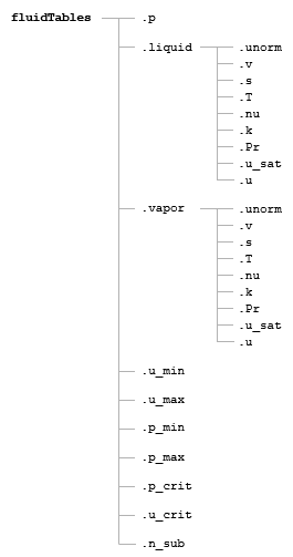
The tables are stored in fluidTables as a structure array. A liquid substructure contains the data for the Liquid Properties tab and a vapor substructure contains that for the Vapor Properties tab. The fields of the substructures contain the fluid properties themselves—specific volume, specific entropy, kinematic viscosity, thermal conductivity, and others needed for simulation.

The tabulated data is in the two-dimensional space of block. A normalized specific internal energy varies across the rows, and absolute pressure varies across the columns. These variables have the special property that, when plotted against them, phase boundaries are vertical and straight, and block calculations are simpler and faster.

Normalized specific internal energy spans between the bounds in uRange across mLiquid rows for the liquid phase and mVapor rows for the vapor phase. Pressure spans between the bounds in pRange across n rows for both liquid and vapor phases. The properties of liquid-vapor mixtures are determined by interpolation between the pure phases.

twoPhaseFluidTables(block,fluidTables) assigns the properties stored in the structure array fluidTables to the parameters of the Two-Phase Fluid Properties (2P) block in the path block. Use the alternative syntax of this function if necessary to generate fluidTables.

Examples

Retrieve the Properties of Water from REFPROP

Get the properties of water from REFPROP and save them as tables in a structure named waterTables. Assume the REFPROP root folder to be C:\REFPROP.

Specify a specific internal energy range of 25-4,000 kJ/kg split over 25 rows and a pressure range of 0.01-15 MPa split over 60 columns:

waterTables = twoPhaseFluidTables([25,4000],[0.01,15],25,25,60,...
'water','C:\Program Files\REFPROP\')

Retrieve the Properties of R-134a from CoolProp

Get the properties of R-134a from CoolProp and save them as tables in a structure named r134aTables. Assume the CoolProp root folder to be C:\CoolProp.

Specify a specific internal energy range of 80-500 kJ/kg split over 25 rows and a pressure range of 0.001-3 MPa split over 60 columns:

r134aTables = twoPhaseFluidTables([80,500],[0.001,3],25,25,60,...
'R134a','py.CoolProp.CoolProp.PropsSI')

Assign the Properties of R-134a to a Block

Populate the parameter fields of a Two-Phase Fluid Properties (2P) block with the property tables of R-134a (stored previously in the structure r134aTables).

Select the block and get its path name:

gcb

Assign to the block the tables of R-134a:

twoPhaseFluidTables(gcb,r134aTables)

Open the block dialog box and check that the parameter fields are specified in terms of r134aTables data.

Input Arguments

uRange — Lower and upper bounds of the specific internal energy range

two-element array in units of kJ/kg

Lower and upper bounds of the specific internal energy range onto which to map the fluid properties. The liquid tables range in specific internal energy from the lower bound to the liquid saturation value. The vapor properties range from the vapor saturation value to the upper bound. The bounds must encompass a range broad enough to include both liquid and vapor saturation values (both retrieved from the database).

Example: [30,4000]

pRange — Lower and upper bounds of the absolute pressure range

two-element array in units of MPa

Lower and upper bounds of the (absolute) pressure range onto which to map the fluid properties. The upper bound can be above the critical pressure of the fluid.

Example: [0.01,100]

mLiquid — Number of rows to include in the liquid tables

unitless scalar

Number of rows to include in the fluid tables for the liquid phase. Each row gives the fluid properties at a fixed value of the normalized specific internal energy, with the normalized specific internal energy increasing from left to right between the lower bound of uRange and the liquid saturation value.

Example: 25

mVapor — Number of rows to include in the vapor tables

unitless scalar

Number of rows to include in the fluid tables for the vapor phase. Each row gives the fluid properties at a fixed value of the normalized specific internal energy, with the normalized specific internal energy increasing from left to right between the vapor saturation value and the upper bound of uRange.

Example: 25

n — Number of columns to include in the fluid tables

unitless scalar

Number of columns to include in the fluid tables. Each column gives the fluid properties at a fixed pressure, with the pressure increasing form left to right between the bounds given in pRange. The number of columns is the same whether for the liquid or vapor phase.

Example: 60

substance — Database name for the fluid whose properties to retrieve

string scalar or character vector

Name of the fluid whose property tables the function is to construct. The name must be one recognized by the database specified. Refer to the database documentation for a list of valid fluid names.

Example: 'water'

installPath — File path to REFPROP installation folder or Python package path to CoolProp PropsSI function

string scalar or character vector

File path to the installation folder for REFPROP or Python package path to the CoolProp PropsSI function. If you are using CoolProp version 6.1.0 or earlier, then InstallPath is the file path to the folder in which the CoolProp MEX files are stored.

Example: 'C:\Program Files\REFPROP\'

Example: 'py.CoolProp.CoolProp.PropsSI'

block — Simulink path to the block to which to assign the fluid tables

string scalar or character vector

Simulink path to the Two-Phase Fluid Properties (2P) block whose fluid tables the function is to specify. To obtain the path to a block, click the block in the model canvas and, at the MATLAB command prompt, enter gcb.

Example: 'TwoPhaseFluidRefrigeration/Two-Phase Fluid Properties (2P)'

fluidTables — Name of the structure array in which the fluid tables are stored

string scalar or character vector

Name of the structure array in which the fluid tables that the function is to specify are stored. The tables must have been generated in a prior call to this function. The structure array must be currently in the MATLAB workspace.

Example: 'waterTables'

Output Arguments

fluidTables — Name of the structure in which to save the fluid tables

structure array

Name of the structure array in which to save the fluid property tables. The array reflects in its hierarchy the structure of the Two-Phase Fluid Properties (2P) block.

Contents of the fluidTables Structure Array

See the table for more on the fields of the fluidTables structure array.

Field	Contents	Dimensions	Units
p	Pressure	n-by-1	MPa
unorm	Normalized specific internal energy	mLiquid- or mVapor-by-1	1
v	Specific volume	mLiquid- or mVapor-by-n	m^3/kg
s	Specific entropy	mLiquid- or mVapor-by-n	kJ/(kg*K)
T	Temperature	mLiquid- or mVapor-by-n	K
nu	Kinematic viscosity	mLiquid- or mVapor-by-n	mm^2/s
k	Thermal conductivity	mLiquid- or mVapor-by-n	W/(m*K)
Pr	Prandtl number	mLiquid- or mVapor-by-n	1
u_sat	Saturation specific internal energy	mLiquid- or mVapor-by-1	kJ/kg
u	Specific internal energy	mLiquid- or mVapor-by-1	kJ/kg
u_min	Minimum specific internal energy	1-by-1	kJ/kg
u_max	Maximum specific internal energy	1-by-1	kJ/kg
p_min	Minimum pressure	1-by-1	MPa
p_max	Maximum pressure	1-by-1	MPa
p_crit	Critical pressure	1-by-1	MPa
u_crit	Specific internal energy at the critical point	1-by-1	kJ/kg
n_sub	Number of elements in the pressure vector below the critical pressure	1-by-1	1

Tips

Install REFPROP as described by NIST (https://www.nist.gov/srd/refprop). The root folder should contain a DLL file and a subfolder with FLD files—the fluid definitions. Only the 64-bit Windows version of REFPROP is supported. This function has been tested with REFPROP versions 9.1, 9.1.1, and 10.

Install CoolProp as described by the CoolProp development team (http://www.coolprop.org/coolprop/wrappers/MATLAB/). CoolProp version 6.2 uses a Python wrapper and requires that you install Python prior to use. For more information, see Configure Your System to Use Python. CoolProp is compatible with Windows, Linux, and Macintosh systems. twoPhaseFluidTables has been tested with CoolProp versions 6.0.0, 6.1.0, and 6.2.0.

Version History

Introduced in R2015b