Multirate Output Feedback Control of Rotary Flexible Link System

R2026b

Since R2026b

This example shows how to control a rotary flexible link system using a multirate output feedback (MOF) approach where the rate at which the output is sampled is different from the rate at which the control input is applied. The example also shows how to estimate the system states by combining the asynchronously sampled output data with the control inputs. The controller uses these estimated states to achieve the desired system performance. This multirate configuration closely resembles practical digital-control scenarios where output sensing and actuation occur asynchronously.

Additionally, this example shows the implementation of an observer-based control strategy where you estimate the system states using a Kalman filter.

Rotary Flexible Link System

In the rotary flexible link system, the base of the flexible link is mounted on the load gear of the rotary servo system. The control input for the system is the servo motor voltage $V$. This voltage generates a torque $$\tau$$ at the load gear of the servo, which in turn rotates the base of the link. This servo experiences viscous friction, characterized by the coefficient $B_{eq}$, which opposes the applied torque at the load gear. The servo has a moment of inertia $J_{eq}$ about the pivot joint.

The flexible link is modeled as a linear spring with stiffness $K_s$ and is subject to viscous damping, characterized by the coefficient $B_l$. This link has a total length $L_l$, a mass $m_l$, and a moment of inertia $J_l$ about the pivot joint.

When the control input is negative, that is, $V<0$, the servo and the flexible link rotate in the clockwise direction due to the resulting torque. Consequently, the servo angle $\theta$ and the deflection angle of the link $\alpha$ decrease. In this example, you design a controller to achieve these objectives:

• Control the servo position to track a desired reference angle.

• Minimize the deflection of the flexible link as the servo changes positions.

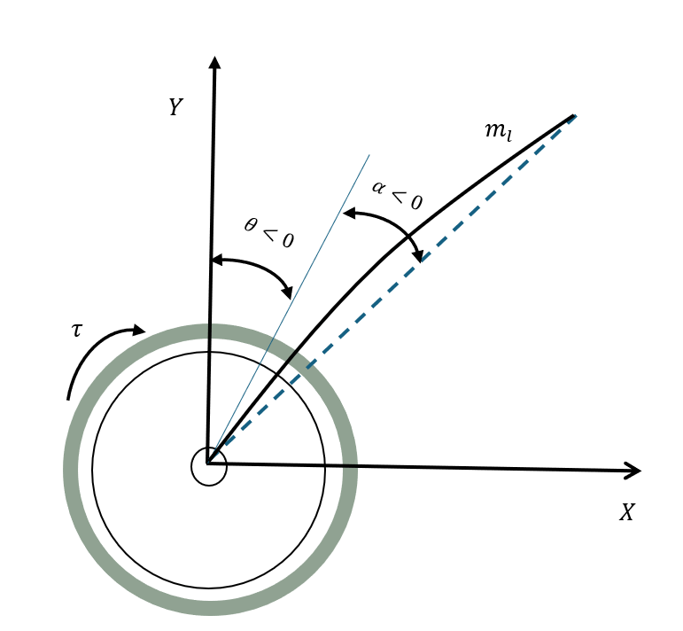
These are the values for the parameters of the rotary flexible link system.

Parameter	Value
$$B_{eq}$$	0.004 $\frac{Nm}{rad/s}$
$$J_{eq}$$	2.08e-3 ${kgm}^2$
$$m_l$$	0.065 $kg$
$$L_l$$	0.419 $m$
$$K_s$$	1.71 $Nm/rad$
$$J_l$$	0.00381 ${kgm}^2$

The state $x$ and output $y$ variables of this system are defined as

$\begin{array}{l}x=\left[\begin{array}{c}\theta \\ \alpha \\ \underset{}{\overset{\dot{}}{\theta }}\\ \underset{}{\overset{\dot{}}{\alpha }}\end{array}\right]\\ y=\left[\begin{array}{c}\theta \\ \alpha \end{array}\right]\end{array}$, where

• $\theta$ is the servo angular position.

• $\underset{}{\overset{\dot{}}{\theta }}$ is the servo angular velocity.

• $\alpha$ is the link deflection angle.

• $\underset{}{\overset{\dot{}}{\alpha }}$ is the rate of link deflection.

The control input $u$ is the servo motor voltage $V$. The dynamics of the system in the state-space form is given by

$$\begin{array}{l}\underset{}{\overset{\dot{}}{x}}=Ax+Bu\\ y=Cx+Du\end{array}$$, where

$$A=\left[\begin{array}{cccc}0& 0& 1& 0\\ 0& 0& 0& 1\\ 0& \frac{K_s}{J_{eq}}& -\frac{B_{eq}}{J_{eq}}& 0\\ 0& -\frac{K_s(J_l+J_{eq})}{J_l{J}_{eq}}& \frac{B_{eq}}{J_{eq}}& 0\end{array}\right]$$, $$B=\left[\begin{array}{c}0\\ 0\\ \frac{1}{J_{eq}}\\ -\frac{1}{J_{eq}}\end{array}\right]$$, $$C=\left[\begin{array}{cccc}1& 0& 0& 0\\ 0& 1& 0& 0\end{array}\right]$$, $$D=\left[\begin{array}{c}0\\ 0\end{array}\right]$$.

To create this rotary flexible link system, first specify all parameter values. Then, calculate the matrices $A$, $B$, $C$, and $D$. You will use these matrices later in this workflow.

Beq  = 0.004;    % N.M/(rad/s)
Jeq  = 2.08e-3;  % Kg.m^2
ml   = 0.065;    % Kg
Ll   = 0.419;    % m
Ks   = 1.71;     % Nm/rad
Jl   = 0.00381;  % Kg.m^2 

A=[0 0 1 0;0 0 0 1;0 Ks/Jeq -Beq/Jeq 0;0 -Ks*(Jl+Jeq)/(Jl*Jeq) Beq/Jeq 0];
B=[0;0;1/Jeq;-1/Jeq];
C=[1 0 0 0;0 1 0 0];
D=[0;0];

Fast Output Sampling Based Control

One technique for MOF control is fast output sampling (FOS). In FOS, the rate at which you sense the output is faster than the rate at which you apply the control input.

You can use FOS only with a system that is both controllable and observable. The system used in this example is controllable and observable.

If you use different parameter values, then to proceed further with this workflow, first check whether the system is controllable and observable by using the rank command.

if rank((ctrb(A,B)))~=4
    disp("The system is not controllable. This method cannot be used.");
end
if rank(obsv(A,C))~=4
    disp("The system is not observable. This method cannot be used.");
end

Calculate States

A discrete-time system sampled at $$\tau$$ seconds is given by:

$$\begin{array}{l}x(k+1)=G_{1}x(k)+H_{1}u(k)\\ y(k)=Cx(k)\end{array}$$

Similarly, a discrete-time system sampled at $$\delta$$ seconds is given by:

$$\begin{array}{l}x(k+1)=G_{2}x(k)+H_{2}u(k)\\ y(k)=Cx(k)\end{array}$$

Here, $G_1$ and $G_2$ are system matrices and $H_1$ and $H_2$ are input matrices for the corresponding systems.

The combined discrete-time MOF system is represented as:

$$\begin{array}{l}x(k+1)=G_{1}x(k)+H_{1}u(k)\\ y(k+1)=C_{0}x(k)+D_{0}u(k)\end{array}$$, where $$y(k)=\left[\begin{array}{c}y((k-1)\tau )\\ y((k-1)\tau +\delta )\\ .\\ .\\ y(k\tau -\delta )\end{array}\right]$$ is a column vector containing N outputs from sampling time $$(k-1)\tau$$ to $$k\tau -\delta$$,

$$C_0=\left[\begin{array}{c}C\\ C{G}_2\\ .\\ .\\ C{G}_2^{N-1}\end{array}\right]$$, and $$D_0=\left[\begin{array}{c}0\\ C{H}_2\\ .\\ .\\ C{\Sigma }_{i=0}^{N-2}{G}_2^i{H}_2\end{array}\right]$$.

The states of the system are represented as a function of past control and present output column vector as

$$x(k)=L_{y}y(k)+L_{u}u(k-1)$$, where

$$L_y=G_1(C_0^T{C}_0{)}^{-1}{C}_0^T$$ and $$L_u=H_1-L_y{D}_0$$.

To represent the states in this form, first create a continuous-time state-space model object using ss (Control System Toolbox).

plantConts=ss(A,B,C,D);

Then, discretize the defined continuous state-space system using c2d (Control System Toolbox). Apply the control input every $$\tau =0.001$$ seconds and sample the output every $$\delta$$ seconds, where $$\delta$$=$$\tau$$/$N$ and $N$is a number greater than or equal to the observability index of the system. For this example, specify $N$ as 4. Obtain two discrete-time systems using two different sample times.

tau=0.001;
N=4;
delta=tau/N;
plantDiscreteTau=c2d(plantConts,tau);
plantDiscreteDelta=c2d(plantConts,delta); 

Extract the state and input-to-state matrices from both of the discretized systems.

G1=plantDiscreteTau.A;
H1=plantDiscreteTau.B;
G2=plantDiscreteDelta.A;
H2=plantDiscreteDelta.B;

Finally, calculate the matrices $C_0$ and $D_0$ and in turn calculate $L_y$ and $L_u$.

C0=[C;C*G2;C*G2*G2;C*G2*G2*G2];
D0=[zeros(size(C,1),1);C*H2;C*G2*H2;C*G2^2*H2];
Ly=G1*inv(C0'*C0)*C0';
Lu=H1-(Ly*D0);

Design Controller

To design a linear-quadratic regulator (LQR) controller, calculate the optimal gain matrix Kf of the closed-loop system by using lqr (Control System Toolbox).

Q=diag([1.8 1 1 0.1]);
R=1;
Kf=lqr(A,B,Q,R);

Simulate Model

To activate FOS in the Simulink® model, set the variant parameter FastOutputSwitchingControl to 1 and the variant parameter ObserverbasedControl to 0.

FastOutputSwitchingControl=1;
ObserverbasedControl=0;  

Open the model. Specify the solver type by using the SolverType configuration parameter. Update the model by using the SimulationCommand configuration parameter.

open_system("flexibleManipulatorMROF.slx");
set_param("flexibleManipulatorMROF","SolverType","Fixed-step");
set_param("flexibleManipulatorMROF","SimulationCommand","update");

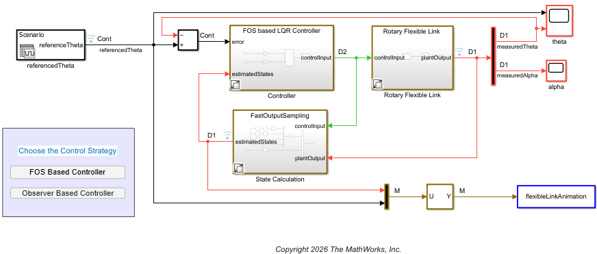
This model calculates states using FOS. The output and control input are sampled at different rates. The model shows the difference in the rates using different colors and labels. It shows the output sensing rate using red with the label D1. It shows the control input rate using green with the label D2. The error in $$\theta$$ is measured continuously.

The FOS-based LQR Controller subsystem uses the gain $K=K_f$. The sample time for the control input is set to $$\tau$$ seconds.

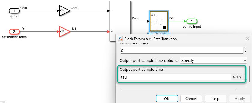
In the Rotary Flexible Link subsystem, the sample time of the plant output is set to $$\delta$$ seconds, which is different from the sample time of the control input.

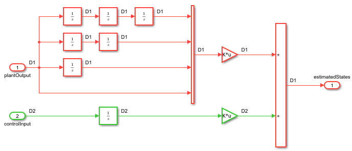
The State Calculation subsystem estimates the states by using FOS. The subsystem uses ${K=L}_y$ as the gain for the plant output and ${K=L}_u$ as the gain for the control input.

Simulate the model.

out= sim("flexibleManipulatorMROF.slx");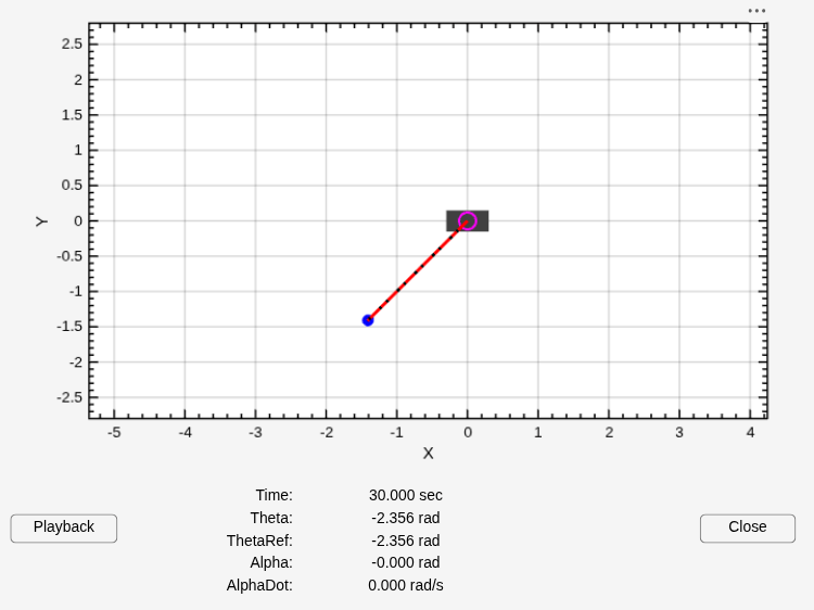

In the Rotary Flexible Link Manipulator animation, the red dotted line represents the servo reference angle $$\theta$$. The blue line represents the flexible link and the black line represents how the link would behave if it were a rigid body.

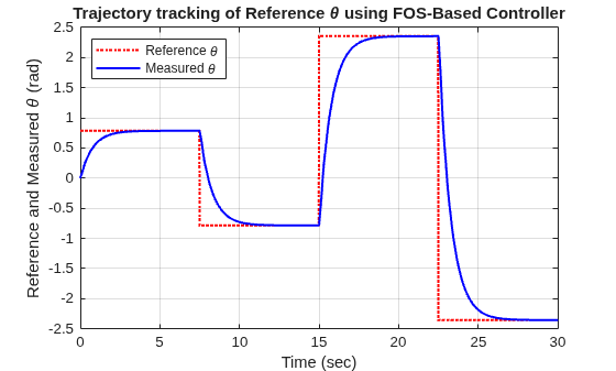
Plot the servo reference angle $\theta$ and the measured output angle $\theta$ over time by using the stairs command. The FOS-based controller tracks the reference angle well.

figure;
stairs(out.tr.time,out.tr.signals(1).values,"r:",LineWidth=1.5);
hold on;
stairs(out.tr.time,out.tr.signals(2).values,"b",LineWidth=1.5);
grid on;
axis([0 30 -2.5 2.5]);
xlabel("Time (sec)");
ylabel("Reference and Measured \theta (rad)");
legend("Reference \theta","Measured \theta",Location="northwest");
title("Trajectory tracking of Reference \theta using FOS-Based Controller");

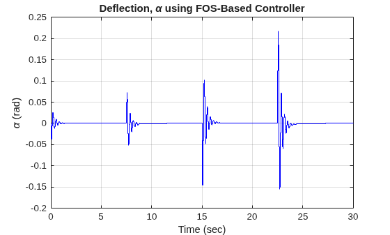
Plot the measured output angle $\alpha$. Whenever the servo angle changes, the deflection angle $\alpha$ increases temporarily before the controller reduces it back to zero.

figure;
stairs(out.alpha.time,out.alpha.signals.values,"b");
grid on;
xlabel("Time (sec)");
ylabel("\alpha (rad)");
title("Deflection, \alpha using FOS-Based Controller");

Compare the measured output states $$\theta$$ and $$\alpha$$ with the estimated states $$\theta$$ and $$\alpha$$.

figure;
tiledlayout(2,1);
nexttile;
stairs(out.logsout{1}.Values.Time,out.logsout{1}.Values.Data(:,1),"b",LineWidth=1.5);
hold on;
stairs(out.logsout{2}.Values.Time,out.logsout{2}.Values.Data(:,1),"r:",LineWidth=1.5);
grid on;
xlabel("Time in Seconds");
ylabel("Measured \theta and Estimated \theta");
legend("Measured \theta","Estimated \theta",Location="southwest");
title("Estimation of \theta using FOS");
hold off;
nexttile;
stairs(out.logsout{1}.Values.Time,out.logsout{1}.Values.Data(:,2),"b",LineWidth=1.5);
hold on;
stairs(out.logsout{2}.Values.Time,out.logsout{2}.Values.Data(:,2),"r:",LineWidth=1.5);
grid on;
xlabel("Time in Seconds");
ylabel("Measured \alpha and Estimated \alpha");
axis([0 30 -0.3 0.3]);
legend("Measured \alpha","Estimated \alpha",Location="southwest");
title("Estimation of deflection \alpha using FOS");
hold off;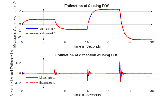

For both $$\theta$$ and $$\alpha$$, the estimated state closely aligns with the measured output state, so the estimated state is accurate.

Observer Based Control

In contrast to FOS, in the observer-based control strategy, you continuously sample the output and control input and estimate the states by using a state observer.

Calculate States

In this control strategy, you estimate states by using a Kalman filter, which serves as a state observer. For more information, see Kalman Filter (Control System Toolbox).

Design Controller

To design a linear-quadratic regulator (LQR) controller, calculate the optimal gain matrix Ko of the closed-loop system using lqr (Control System Toolbox).

Ko=lqr(A,B,Q,R);

Simulate Model

To activate observer-based control in the Simulink model, set the variant parameter FastOutputSwitchingControl to 0 and the variant parameter ObserverbasedControl to 1.

FastOutputSwitchingControl = 0;
ObserverbasedControl = 1;

Open the model. Specify the solver type and update the model.

set_param("flexibleManipulatorMROF","SolverType","Variable-step");
set_param("flexibleManipulatorMROF","SimulationCommand","update");

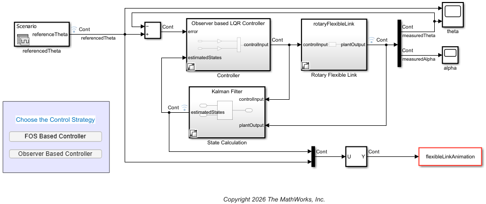
This model calculates states using a Kalman filter. The plant output, the control input, and the error in the servo angle $$\theta$$ are all sampled continuously.

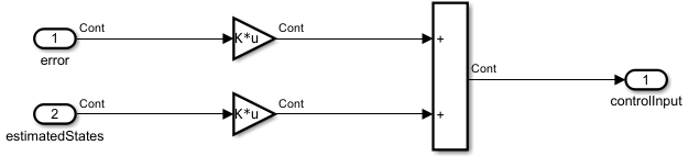
The observer-based LQR Controller subsystem uses the gain $K=K_o$.

In the Rotary Flexible Link subsystem, the control input and the plant output are both sampled continuously, as reflected in the top-level Simulink model.

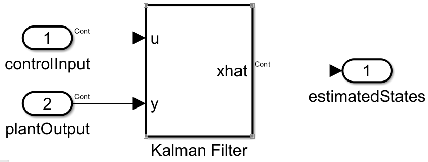
The State Calculation subsystem estimates the states using a Kalman Filter block.

Simulate the model.

out1= sim("flexibleManipulatorMROF.slx");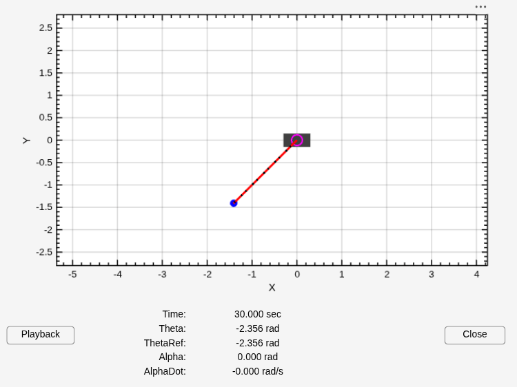

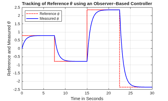
Plot the servo reference angle $\theta$ and the measured output angle $\theta$ over time using the stairs command. The observer-based controller tracks the reference servo angle well.

figure;
stairs(out1.tr.time,out1.tr.signals(1).values,"r:",LineWidth=1.5);
hold on;
stairs(out1.tr.time,out1.tr.signals(2).values,"b",LineWidth=1.5);
grid on;
axis([0 30 -2.5 2.5]);
xlabel("Time in Seconds");
ylabel("Reference and Measured \theta");
legend("Reference \theta","Measured \theta",Location="northwest");
title("Tracking of Reference \theta using an Observer–Based Controller");

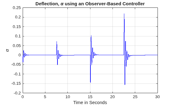
Plot the measured output angle $\alpha$. Whenever the servo angle changes, the deflection angle $\alpha$ increases temporarily before the controller reduces it back to zero.

figure;
stairs(out1.alpha.time,out1.alpha.signals.values,"b");
grid on;
xlabel("Time in Seconds");
ylabel("\alpha");
title("Deflection, \alpha using an Observer-Based Controller");

Compare the measured output states $$\theta$$ and $$\alpha$$ with the estimated states $$\theta$$ and $$\alpha$$. The measured and estimated states are almost the same, which indicates that the Kalman filter estimates the states accurately.

figure;
tiledlayout(2,1);
nexttile;
stairs(out1.logsout{1}.Values.Time,out1.logsout{1}.Values.Data(:,1),"b:",LineWidth=1.5);
hold on;
stairs(out1.logsout{2}.Values.Time,out1.logsout{2}.Values.Data(:,1),"r:",LineWidth=1.5);
grid on;
xlabel("Time in Seconds");
ylabel("Measured \theta and Estimated \theta");
legend("Measured \theta","Estimated \theta",Location="southwest");
title("Estimation of \theta using an Observer–Based Controller");
hold off;
nexttile;
stairs(out1.logsout{1}.Values.Time,out1.logsout{1}.Values.Data(:,2),"b:",LineWidth=1.5);
hold on;
stairs(out1.logsout{2}.Values.Time,out1.logsout{2}.Values.Data(:,2)',"r:",LineWidth=1.5);
grid on;
axis([0 30 -0.3 0.3]);
xlabel("Time in Seconds");
ylabel("Measured \alpha and Estimated \alpha");
legend("Measured \alpha","Estimated \alpha",Location="southwest");
title("Estimation of deflection \alpha using an Observer–Based Controller");
hold off;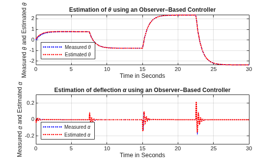

Comparison of Both Approaches

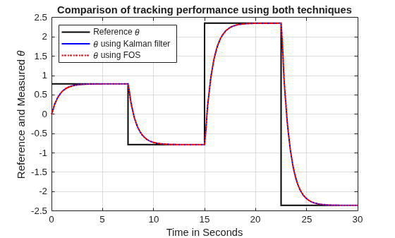
Plot the following over time: the reference $$\theta$$, the $$\theta$$ that you measured using FOS-based control, and the $$\theta$$ that you measured using observer-based control. Compare how the two techniques perform at tracking the reference $$\theta$$.

figure;
stairs(out1.tr.time,out1.tr.signals(1).values,"k",LineWidth=1.5);
hold on;
stairs(out1.tr.time,out1.tr.signals(2).values,"b",LineWidth=1.5);
stairs(out.tr.time,out.tr.signals(2).values,"r:",LineWidth=1.5);
grid on;
axis([0 30 -2.5 2.5]);
xlabel("Time in Seconds");
ylabel("Reference and Measured \theta");
legend("Reference \theta","\theta using Kalman filter","\theta using FOS",Location="northwest");
title("Comparison of tracking performance using both techniques");

Plot the following over time: the deflection $$\alpha$$ that you measured using FOS-based control, and the deflection $$\alpha$$ that you measured using observer-based control. Compare how the two techniques perform at bringing the deflection back to 0.

figure;
stairs(out1.alpha.time,out1.alpha.signals.values,"b",LineWidth=1.5);
hold on;
stairs(out.alpha.time,out.alpha.signals.values,"r:",LineWidth=1.5);
grid on;
axis([0 30 -0.3 0.3]);
xlabel("Time in Seconds");
ylabel("\alpha");
legend("\alpha using Kalman filter","\alpha using FOS",Location="northwest");
title("Comparison of deflection performance using both techniques");

Both the techniques perform well at tracking the reference angle and bringing the deflection back to 0. The primary distinction between both these approaches lies in state estimation. The observer in FOS uses multirate simulation to estimate the system states in finite time while the Kalman filter achieves state estimation only asymptotically.

References

[1] Janardhanan, S., and B. Bandyopadhyay. “Discrete Sliding Mode Control of Systems With Unmatched Uncertainty Using Multirate Output Feedback.” IEEE Transactions on Automatic Control 51, no. 6 (2006): 1030–35. https://doi.org/10.1109/TAC.2006.876810.