Estimate Lookup Table Values from Data

Objectives

This example shows how to estimate lookup table values from time-domain input-output (I/O) data in the Parameter Estimator.

About the Data

In this example, use the I/O data in lookup_regular.mat to estimate the values of a lookup table. The MAT file includes the following variables:

xdata1 — Consists of 63 uniformly-sampled input data points in the range [0,6.5]
ydata1 — Consists of output data corresponding to the input data samples
time1 — Time vector

Use the I/O data to estimate the lookup table values in the lookup_regular Simulink^® model. The lookup table in the model contains ten values, which are stored in the MATLAB^® variable table. The initial table values comprise a vector of 0s. To learn more about how to model a system using lookup tables, see Guidelines for Choosing a Lookup Table.

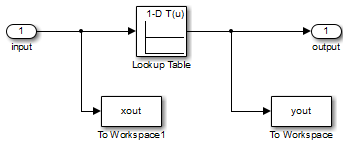
Lookup Table Estimation Model

Open Live Script

Open the lookup table model.

open_system('lookup_regular.slx')

This command opens the Simulink® model, and loads the estimation data into the MATLAB® workspace.

Simulink model with Lookup Table

Open a Parameter Estimation Session

To estimate the lookup table values, open a parameter estimation session.

In the Simulink model, select Parameter Estimator from the Apps tab, in the gallery, under Control Systems to open a new session with name lookup_regular in the Parameter Estimator.

Parameter Estimator app main window. Parameter Estimation toolstrip is on the top. Parameters, Experiments, Results, and Preview panes are on the left, from top to bottom.

Estimate the Table Values Using Default Settings

Use the following steps to estimate the lookup table values.

Create a new experiment by clicking New Experiment on the Parameter Estimation tab. Name it EstimationData. Then import the I/O data, xdata1 and ydata1, and the time vector, time1, into the experiment. To do this open the experiment editor by right-clicking EstimationData and selecting Edit.... Type [time1,ydata1] in the output dialog box and [time1,xdata1] in the input dialog box in the experiment editor. For more information, see Import Data for Parameter Estimation. After you import the data the experiment looks as follows:
Run an initial simulation to view the I/O data, simulated output, and the initial table values. To do so, type the following commands at the MATLAB prompt:
```
sim('lookup_regular')
figure(1)
plot(xdata1,ydata1,'m*',xout, yout,'b^')
hold on
plot(linspace(0,6.5,10),table,'k','LineWidth',2);
legend('Measured data',...
    'Initial simulation data',...
    'Initial table values');
```
The x-axis and y-axis of the figure represent the input and output data, respectively. The figure shows the following plots:
- Measured data — Represented by the magenta stars (*).
- Initial table values — Represented by the black line.
- Initial simulation data — Represented by the blue deltas (Δ).
You can see that the initial table values and simulated data do not match with the measured data.
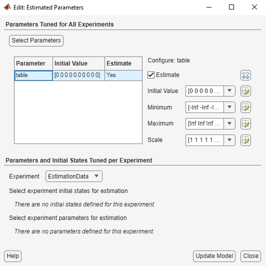
To select the table values to estimate, on the Parameter Estimation tab, click the Select Parameters button to open the Edit:Estimated Parameters dialog box. In the Parameters Tuned for all Experiments panel, click Select parameters to launch the Select Model Variables dialog box. Check the box next to table, and click OK.
The Edit:Estimated Parameters window now looks as follows. The table values are selected for estimation by default.
On the Parameter Estimation tab, click Select Experiments. EstimationData is selected for estimation by default. If not, check the box under the Estimation column, and click Close.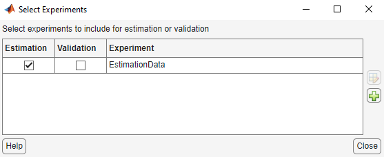
To estimate the table values using the default settings, on the Parameter Estimation tab, click Estimate to open the Parameter Trajectory plot and Estimation Progress Report window. The Parameter Trajectory plot shows the change in the parameter values at each iteration.
After the estimation converges, the Parameter Trajectory plot looks like this:
The Estimation Progress Report shows the iteration number, number of times the objective function is evaluated, and the value of the cost function at the end of each iteration. After the estimation converges, the Estimation Progress Report looks like this:

The estimated parameters are saved in EstimatedParams in the Results section of the data browser pane on the left. To view the results, right-click on EstimatedParams and then select Open. The report resembles the following.

This report includes the estimated parameter values, the final value of the cost function, and other optimization results. You can see that the optimization stopped when the size of the gradient, 1.18e-14 was less than the criteria value, 1e-3.

Validate the Estimation Results

After you estimate the table values, as described in Estimate the Table Values Using Default Settings, you must use another data set to validate that you have not over-fitted the model. You can plot and examine the following plots to validate the estimation results:

Residuals plot
Measured and simulated data plots

To validate the estimation results:

Create a new experiment to use for validation. Name it ValidationData. Import the validation I/O data, xdata2 and ydata2, and time vector, time2 in the ValidationData experiment. To do this open the experiment editor by right-clicking ValidationData and selecting Edit.... Then, type [time2,ydata2] in the output dialog box and [time2,xdata2] in the input dialog box in the experiment editor. For more information, see Import Data for Parameter Estimation.
To select the experiment for validation, on the Parameter Estimation tab, click Select Experiments. The ValidationData experiment is selected for estimation by default. Deselect the box for estimation and check it for validation.
To select results to use, on the Validation tab, click Select Results to Validate. Deselect Use current parameter values and select EstimatedParams, and click OK.
The Parameter Estimator, by default, displays the experiment plot after validation. Add the residuals plot by checking the corresponding box on the Validation tab.

To start validation, on the Validation tab, click Validate.
Examine the plots
1. Experiment plot
  You can see that the data simulated using the estimated parameters agrees with the measured validation data.
2. Click Residual plot: ValidationData to open the residuals plot.
  The residuals, which show the difference between the simulated and measured data, lie in the range [-0.15,0.15]— within 15% of the maximum output variation. This indicates a good match between the measured and the simulated table data values.
3. Plot and examine the estimated table values against the validation data set and the simulated table values by typing the following commands at the MATLAB prompt.
  sim('lookup_regular') figure(2); plot(xdata2,ydata2, 'm*', xout, yout,'b^') hold on; plot(linspace(0,6.5,10), table, 'k', 'LineWidth', 2)
  The plot shows that the table values, displayed as the black line, match both the validation data and the simulated table values. The table data values cover the entire range of input values, which indicates that all the lookup table values have been estimated.