Model Ferrite Core Using Magnetic Core Block

Since R2025a

This example shows how to adjust the Jiles-Atherton parameters to obtain a good fit for the B-H curve of a magnetic core. The Magnetic Core block uses the Jiles-Atherton model to define the relationship between the magnetic flux density, B, and the total field strength, H. You can parametrize the block by specifying the Jiles-Atherton parameters directly. Alternatively, you can parameterize the block using saturated B-H curve data or by specifying magnetic characteristics. If you do not specify the Jiles-Atherton parameters directly, the block estimates the Jiles-Atherton parameters based on the assumption that you have a saturated iron core. This estimate is not always accurate for other types of core, such as ferrites with small values of coercivity and remanence. Always check that the B-H curve the block uses matches your input data.

In this example, you model a ferrite core that a controlled flux source magnetizes. You obtain an initial estimate of the Jiles-Atherton parameters for the ferrite core by parameterizing the Magnetic Core block with a saturated B-H curve. Then, you examine the predicted B-H curve and adjust the Jiles-Atherton parameters to get a better fit with your data.

Open Model

Open the modelFerriteCoreUsingMagneticCoreBlock model.

myModel = "modelFerriteCoreUsingMagneticCoreBlock";
open_system(myModel);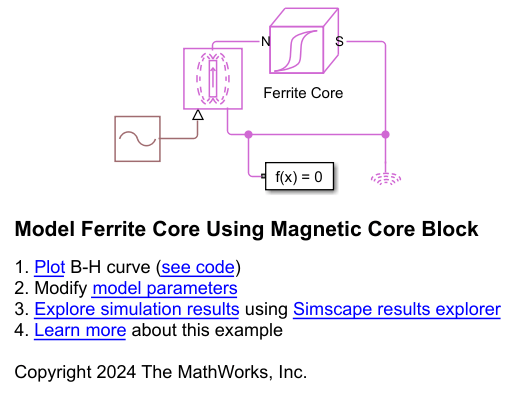

Import B-H Curve and Plot Initial Simulation Results

Start by obtaining an estimate of the Jiles-Atherton parameters by parameterizing the block with the saturated B-H curve. Set the Parameterization option parameter to Saturated B-H curve, simulate the model, and plot the results. For more information about parameterizing cores from saturated B-H curves, see the Parameterize Magnetic Core Block Using B-H Curve Data example.

load("modelFerriteCoreUsingMagneticCoreBlock.mat");
set_param(strcat(myModel,"/Ferrite Core"),parameterization_option="ee.enum.passive.parameterizationOption.BH");
modelFerriteCoreUsingMagneticCoreBlockPlotCurve;

 The Jiles-Atherton parameters used for the simulation are: 
 Ms = 300645.6524A/m 
 a = 10.5294A/m 
 alpha = 2.9852e-05 
 c = 0.001727 
 k = 10A/m 

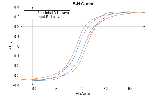
In most cases, the Magnetic Core block generates a B-H curve very close to the input curve. However, in this example with a ferrite core, the estimated Jiles-Atherton parameters do not generate a curve that overlaps with the input data. The simulated B-H curve is wider than the input curve, which indicates that the predictions of coercivity and remanence are too high. The simulated B-H curve also saturates at a lower magnitude of flux density and a larger magnitude of field intensity.

MATLAB® displays the estimated Jiles-Atherton parameters at the beginning of the simulation. Assign these initial estimates to workspace variables.

 Ms = 300645.6524; % A/m
 a = 10.5294; % A/m
 alpha = 2.9852e-05; 
 c = 0.001727; 
 k = 10; % A/m 

Adjust Jiles-Atherton Parameters Manually

Now adjust the Jiles-Atherton parameters manually to obtain a better fit for the B-H curve. Liu et al. [1] explain the effects of modifying each of the parameters independently and provide recommendations on how to adjust them.

• The saturation magnetization, $$Ms$$, defines the maximum magnetization that the material can achieve. A higher value results in a taller B-H loop.

• The anhysteretic magnetization coefficient, $$a$$, relates to the average energy required to overcome the pinning of domain walls. This variable affects the initial slope and the coercivity of the hysteresis loop. When you increase $$a$$, the saturation magnetization, the slope at coercivity, and the remanence decrease.

• The inter-domain coupling factor, $$\alpha$$, describes the proportion of the magnetization that is reversible. When you increase $$\alpha$$, you get a narrower hysteresis loop, indicating that a larger portion of the magnetization can be reversed without energy loss.

• The coefficient for reversible magnetization, $$c$$, influences the rate at which the magnetization approaches its equilibrium value. When you increase $$c$$, the B-H curve approaches the saturation point more gradually, reducing the slope of the B-H curve. In addition, the coercivity, remanence, and hysteresis decrease.

• The bulk coupling coefficient, $$k$$, affects the shape and width of the hysteresis loop. When you increase $$k$$, you get a wider loop, indicating a greater magnetic remanence and coercivity.

The simulated curve saturates at a lower magnitude of field intensity than expected, and has a higher coercivity and remanence. The simulated curve also approaches saturation more gradually.

Adjusting the Jiles-Atherton parameters is not an exact science because adjusting different parameters can have the same effect on the B-H curve. For example, to decrease the coercivity, you can increase $$a$$ or $$c$$, or decrease $$k$$. Make incremental changes to the variables and verify that these changes have the desired effect. In this example, you implement one of many possible sets of changes that result in better agreement with your input B-H curve.

Increase $$Ms$$ to correct the saturation value.

Ms = Ms * 1.13;

Increase $$a$$ to reduce remanence.

a = a * 1.9;

Increase $$\alpha$$ to reduce the width of the hysteresis loop.

alpha = alpha * 3.4;

Keep $$c$$ the same.

c = c;

Reduce $$k$$ to almost half its value to reduce remanence and coercivity.

k = k / 1.7;

Simulate the model again and plot the simulated B-H curve with the new Jiles-Atherton parameter values.

set_param(strcat(myModel,"/Ferrite Core"),parameterization_option="ee.enum.passive.parameterizationOption.JilesAtherton");
modelFerriteCoreUsingMagneticCoreBlockPlotCurve;

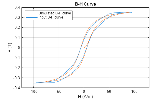
The simulated B-H curve now closely matches the input B-H curve. You can use this model to accurately represent your ferrite core.

References

[1] Liu, Qingsong, Junjie Zhou, Jinwei Chu, Shunliang Wang, Qingming Xin, and Chuang Fu. "Identification of Jiles-Atherton Model Parameters Using Improved Genetic Algorithm." In 2020 IEEE 1st China International Youth Conference on Electrical Engineering (CIYCEE), 1–6, 2020. https://doi.org/10.1109/CIYCEE49808.2020.9332611.