genrfeatures
Syntax
Description
The genrfeatures function enables you to automate the feature
engineering process in the context of a machine learning workflow. Before passing tabular
training data to a regression model, you can create new features from the predictors in the
data by using genrfeatures. Use the returned data to train the regression
model.
genrfeatures allows you to generate features from variables with data
types—such as datetime, duration, and various
int types—that are not supported by most regression model training
functions. The resulting features have data types that are supported by these training
functions.
To better understand the generated features, use the describe function
of the returned FeatureTransformer
object. To apply the same training set feature transformations to a test set, use the
transform function
of the FeatureTransformer object.
[
uses automated feature engineering to create Transformer,NewTbl] = genrfeatures(Tbl,ResponseVarName,q)q features from the
predictors in Tbl. The software assumes that the
ResponseVarName variable in Tbl is the response
and does not create new features from this variable. genrfeatures
returns a FeatureTransformer object (Transformer) and
a new table (NewTbl) that contains the transformed features.
By default, genrfeatures assumes that generated features are used
to train an interpretable linear regression model. If you want to generate features to
improve the accuracy of a bagged ensemble, specify
TargetLearner="bag".
[
assumes that the vector Transformer,NewTbl] = genrfeatures(Tbl,Y,q)Y is the response variable and creates new
features from the variables in Tbl.
[
uses the explanatory model Transformer,NewTbl] = genrfeatures(Tbl,formula,q)formula to determine the response variable
in Tbl and the subset of Tbl predictors from which
to create new features.
[
specifies options using one or more name-value arguments in addition to any of the input
argument combinations in previous syntaxes. For example, you can change the expected learner
type, the method for selecting new features, and the standardization method for transformed
data.Transformer,NewTbl] = genrfeatures(___,Name=Value)
Examples
Use automated feature engineering to generate new features. Train a linear regression model using the generated features. Interpret the relationship between the generated features and the trained model.
Load the patients data set. Create a table from a subset of the variables. Display the first few rows of the table.
load patients
Tbl = table(Age,Diastolic,Gender,Height,SelfAssessedHealthStatus, ...
    Smoker,Weight,Systolic);
head(Tbl)
    Age    Diastolic      Gender      Height    SelfAssessedHealthStatus    Smoker    Weight    Systolic
    ___    _________    __________    ______    ________________________    ______    ______    ________

    38        93        {'Male'  }      71           {'Excellent'}          true       176        124
    43        77        {'Male'  }      69           {'Fair'     }          false      163        109
    38        83        {'Female'}      64           {'Good'     }          false      131        125
    40        75        {'Female'}      67           {'Fair'     }          false      133        117
    49        80        {'Female'}      64           {'Good'     }          false      119        122
    46        70        {'Female'}      68           {'Good'     }          false      142        121
    33        88        {'Female'}      64           {'Good'     }          true       142        130
    40        82        {'Male'  }      68           {'Good'     }          false      180        115
Generate 10 new features from the variables in Tbl. Specify the Systolic variable as the response. By default, genrfeatures assumes that the new features will be used to train a linear regression model.
rng("default") % For reproducibility
[T,NewTbl] = genrfeatures(Tbl,"Systolic",10)
T =
  FeatureTransformer with properties:

                     Type: 'regression'
            TargetLearner: 'linear'
    NumEngineeredFeatures: 10
      NumOriginalFeatures: 0
         TotalNumFeatures: 10
NewTbl=100×11 table
    zsc(d(Smoker))    q8(Age)    eb8(Age)    zsc(sin(Height))    zsc(kmd8)    q6(Height)    eb8(Diastolic)    q8(Diastolic)    zsc(fenc(c(SelfAssessedHealthStatus)))    q10(Weight)    Systolic
    ______________    _______    ________    ________________    _________    __________    ______________    _____________    ______________________________________    ___________    ________

         1.3863          4          5              1.1483         -0.56842        6               8                 8                         0.27312                        7            124
       -0.71414          6          6             -0.3877          -2.0772        5               2                 2                         -1.4682                        6            109
       -0.71414          4          5              1.1036         -0.21519        2               4                 5                         0.82302                        3            125
       -0.71414          5          6             -1.4552         -0.32389        4               2                 2                         -1.4682                        4            117
       -0.71414          8          8              1.1036           1.2302        2               3                 4                         0.82302                        1            122
       -0.71414          7          7             -1.5163         -0.88497        4               1                 1                         0.82302                        5            121
         1.3863          3          3              1.1036          -1.1434        2               6                 6                         0.82302                        5            130
       -0.71414          5          6             -1.5163          -0.3907        4               4                 5                         0.82302                        8            115
       -0.71414          1          2             -1.5163           0.4278        4               3                 3                         0.27312                        9            115
       -0.71414          2          3            -0.26055        -0.092621        3               5                 6                         0.27312                        3            118
       -0.71414          7          7             -1.5163          0.16737        4               2                 2                         0.27312                        2            114
       -0.71414          6          6            -0.26055         -0.32104        3               1                 1                         -1.8348                        5            115
       -0.71414          1          1              1.1483        -0.051074        6               1                 1                         -1.8348                        7            127
         1.3863          5          5             0.14351           2.3695        6               8                 8                         0.27312                        10           130
       -0.71414          3          4             0.96929         0.092962        2               3                 4                         0.82302                        3            114
         1.3863          8          8              1.1483        -0.049336        6               7                 8                         0.82302                        8            130
      ⋮
T is a FeatureTransformer object that can be used to transform new data, and newTbl contains the new features generated from the Tbl data.
To better understand the generated features, use the describe object function of the FeatureTransformer object. For example, inspect the first two generated features.
describe(T,1:2)
                         Type        IsOriginal    InputVariables                          Transformations
                      ___________    __________    ______________    ___________________________________________________________

    zsc(d(Smoker))    Numeric          false           Smoker        Variable of type double converted from an integer data type
                                                                     Standardization with z-score (mean = 0.34, std = 0.4761)
    q8(Age)           Categorical      false           Age           Equiprobable binning (number of bins = 8)
The first feature in newTbl is a numeric variable, created by first converting the values of the Smoker variable to a numeric variable of type double and then transforming the results to z-scores. The second feature in newTbl is a categorical variable, created by binning the values of the Age variable into 8 equiprobable bins.
Use the generated features to fit a linear regression model without any regularization.
Mdl = fitrlinear(NewTbl,"Systolic",Lambda=0);Plot the coefficients of the predictors used to train Mdl. Note that fitrlinear expands categorical predictors before fitting a model.
p = length(Mdl.Beta);
[sortedCoefs,expandedIndex] = sort(Mdl.Beta,ComparisonMethod="abs");
sortedExpandedPreds = Mdl.ExpandedPredictorNames(expandedIndex);
bar(sortedCoefs,Horizontal="on")
yticks(1:2:p)
yticklabels(sortedExpandedPreds(1:2:end))
xlabel("Coefficient")
ylabel("Expanded Predictors")
title("Coefficients for Expanded Predictors")
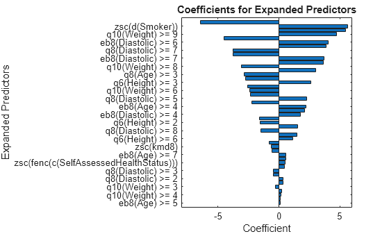
Identify the predictors whose coefficients have larger absolute values.
bigCoefs = abs(sortedCoefs) >= 4;
flip(sortedExpandedPreds(bigCoefs))
ans = 1×6 cell
    {'eb8(Diastolic) >= 5'}    {'zsc(d(Smoker))'}    {'q8(Age) >= 2'}    {'q10(Weight) >= 9'}    {'q6(Height) >= 5'}    {'eb8(Diastolic) >= 6'}
You can use partial dependence plots to analyze the categorical features whose levels have large coefficients in terms of absolute value. For example, inspect the partial dependence plot for the eb8(Diastolic) variable, whose levels eb8(Diastolic) >= 5 and eb8(Diastolic) >= 6 have coefficients with large absolute values. These two levels correspond to noticeable changes in the predicted Systolic values.
plotPartialDependence(Mdl,"eb8(Diastolic)",NewTbl);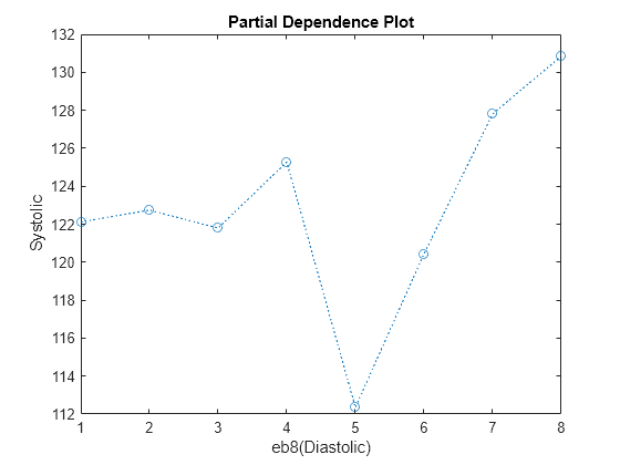
Generate new features to improve the predictive performance of an interpretable linear regression model. Compare the test set performance of a linear model trained on the original data to the test set performance of a linear model trained on the transformed features.
Load the carbig data set, which contains measurements of cars made in the 1970s and early 1980s.
load carbigConvert the Origin variable to a categorical variable. Then create a table containing the predictor variables Acceleration, Displacement, and so on, as well as the response variable MPG. Each row contains the measurements for a single car. Remove rows that have missing values.
Origin = categorical(cellstr(Origin));
cars = table(Acceleration,Displacement,Horsepower, ...
    Model_Year,Origin,Weight,MPG);
Tbl = rmmissing(cars);
Partition the data into training and test sets. Use approximately 70% of the observations as training data, and 30% of the observations as test data. Partition the data using cvpartition.
rng("default") % For reproducibility of the partition
c = cvpartition(size(Tbl,1),Holdout=0.3);

trainIdx = training(c);
trainTbl = Tbl(trainIdx,:);

testIdx = test(c);
testTbl = Tbl(testIdx,:);
Use the training data to generate 45 new features. Inspect the returned FeatureTransformer object.
[T,newTrainTbl] = genrfeatures(trainTbl,"MPG",45);
T
T =
FeatureTransformer with properties:
Type: 'regression'
TargetLearner: 'linear'
NumEngineeredFeatures: 43
NumOriginalFeatures: 2
TotalNumFeatures: 45
Note that T.NumOriginalFeatures is 2, which means the function keeps two of the original predictors.
Apply the transformations stored in the object T to the test data.
newTestTbl = transform(T,testTbl);
Compare the test set performances of a linear model trained on the original features and a linear model trained on the new features.
Train a linear regression model using the original training set trainTbl, and compute the mean squared error (MSE) of the model on the original test set testTbl. Then, train a linear regression model using the transformed training set newTrainTbl, and compute the MSE of the model on the transformed test set newTestTbl.
originalMdl = fitrlinear(trainTbl,"MPG");
originalTestMSE = loss(originalMdl,testTbl,"MPG")
originalTestMSE =
65.9916
newMdl = fitrlinear(newTrainTbl,"MPG");
newTestMSE = loss(newMdl,newTestTbl,"MPG")
newTestMSE =
12.0342
newTestMSE is less than originalTestMSE, which suggests that the linear model trained on the transformed data performs better than the linear model trained on the original data.
Compare the predicted test set response values to the true response values for both models. Plot the predicted miles per gallon (MPG) along the vertical axis and the true MPG along the horizontal axis. Points on the reference line indicate correct predictions. A good model produces predictions that are scattered near the line.
predictedTestY = predict(originalMdl,testTbl);
newPredictedTestY = predict(newMdl,newTestTbl);

plot(testTbl.MPG,predictedTestY,".")
hold on
plot(testTbl.MPG,newPredictedTestY,".")
hold on
plot(testTbl.MPG,testTbl.MPG)
hold off
xlabel("True Miles Per Gallon (MPG)")
ylabel("Predicted Miles Per Gallon (MPG)")
legend(["Original Model Results","New Model Results","Reference Line"])

Use genrfeatures to engineer new features before training a bagged ensemble regression model. Before making predictions on new data, apply the same feature transformations to the new data set. Compare the test set performance of the ensemble that uses the engineered features to the test set performance of the ensemble that uses the original features.
Read power outage data into the workspace as a table. Remove observations with missing values, and display the first few rows of the table.
outages = readtable("outages.csv");
Tbl = rmmissing(outages);
head(Tbl)
Region OutageTime Loss Customers RestorationTime Cause
_____________ ________________ ______ __________ ________________ ___________________
{'SouthWest'} 2002-02-01 12:18 458.98 1.8202e+06 2002-02-07 16:50 {'winter storm' }
{'SouthEast'} 2003-02-07 21:15 289.4 1.4294e+05 2003-02-17 08:14 {'winter storm' }
{'West' } 2004-04-06 05:44 434.81 3.4037e+05 2004-04-06 06:10 {'equipment fault'}
{'MidWest' } 2002-03-16 06:18 186.44 2.1275e+05 2002-03-18 23:23 {'severe storm' }
{'West' } 2003-06-18 02:49 0 0 2003-06-18 10:54 {'attack' }
{'NorthEast'} 2003-07-16 16:23 239.93 49434 2003-07-17 01:12 {'fire' }
{'MidWest' } 2004-09-27 11:09 286.72 66104 2004-09-27 16:37 {'equipment fault'}
{'SouthEast'} 2004-09-05 17:48 73.387 36073 2004-09-05 20:46 {'equipment fault'}
Some of the variables, such as OutageTime and RestorationTime, have data types that are not supported by regression model training functions like fitrensemble.
Partition the data into training and test sets. Use approximately 70% of the observations as training data, and 30% of the observations as test data. Partition the data using cvpartition.
rng("default") % For reproducibility of the partition
c = cvpartition(size(Tbl,1),Holdout=0.30);
TrainTbl = Tbl(training(c),:);
TestTbl = Tbl(test(c),:);
Use the training data to generate 30 new features to fit a bagged ensemble. By default, the 30 features include original features that can be used as predictors by a bagged ensemble.
[Transformer,NewTrainTbl] = genrfeatures(TrainTbl,"Loss",30, ...
    TargetLearner="bag");
Transformer
Transformer =
  FeatureTransformer with properties:

                     Type: 'regression'
            TargetLearner: 'bag'
    NumEngineeredFeatures: 27
      NumOriginalFeatures: 3
         TotalNumFeatures: 30
Create NewTestTbl by applying the transformations stored in the object Transformer to the test data.
NewTestTbl = transform(Transformer,TestTbl);
Train a bagged ensemble using the original training set TrainTbl, and compute the mean squared error (MSE) of the model on the original test set TestTbl. Specify only the three predictor variables that can be used by fitrensemble (Region, Customers, and Cause), and omit the two datetime predictor variables (OutageTime and RestorationTime). Then, train a bagged ensemble using the transformed training set NewTrainTbl, and compute the MSE of the model on the transformed test set NewTestTbl.
originalMdl = fitrensemble(TrainTbl,"Loss ~ Region + Customers + Cause", ...
    Method="bag");
originalTestMSE = loss(originalMdl,TestTbl)
originalTestMSE =
1.8999e+06
newMdl = fitrensemble(NewTrainTbl,"Loss",Method="bag");
newTestMSE = loss(newMdl,NewTestTbl)
newTestMSE =
1.8617e+06
newTestMSE is less than originalTestMSE, which suggests that the bagged ensemble trained on the transformed data performs slightly better than the bagged ensemble trained on the original data.
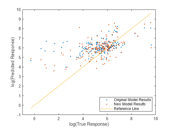
Compare the predicted test set response values to the true response values for both models. Plot the log of the predicted response along the vertical axis and the log of the true response (Loss) along the horizontal axis. Points on the reference line indicate correct predictions. A good model produces predictions that are scattered near the line.
predictedTestY = predict(originalMdl,TestTbl);
newPredictedTestY = predict(newMdl,NewTestTbl);

plot(log(TestTbl.Loss),log(predictedTestY),".")
hold on
plot(log(TestTbl.Loss),log(newPredictedTestY),".")
hold on
plot(log(TestTbl.Loss),log(TestTbl.Loss))
hold off
xlabel("log(True Response)")
ylabel("log(Predicted Response)")
legend(["Original Model Results","New Model Results","Reference Line"], ...
    Location="southeast")
xlim([-1 10])
ylim([-1 10])
Engineer and inspect new features before training a support vector machine (SVM) regression model with a Gaussian kernel. Then, assess the test set performance of the model.
Load the carbig data set, which contains measurements of cars made in the 1970s and early 1980s.
load carbigCreate a table containing the numeric predictor variables Acceleration, Displacement, and so on, as well as the response variable MPG. Each row contains the measurements for a single car. Remove rows that have missing values.
cars = table(Acceleration,Displacement,Horsepower, ...
    Model_Year,Weight,MPG);
Tbl = rmmissing(cars);
head(Tbl)
Acceleration Displacement Horsepower Model_Year Weight MPG
____________ ____________ __________ __________ ______ ___
12 307 130 70 3504 18
11.5 350 165 70 3693 15
11 318 150 70 3436 18
12 304 150 70 3433 16
10.5 302 140 70 3449 17
10 429 198 70 4341 15
9 454 220 70 4354 14
8.5 440 215 70 4312 14
Partition the data into training and test sets. Use approximately 75% of the observations as training data, and 25% of the observations as test data. Partition the data using cvpartition.
rng("default") % For reproducibility of the partition
n = length(Tbl.MPG);
c = cvpartition(n,Holdout=0.25);
trainTbl = Tbl(training(c),:);
testTbl = Tbl(test(c),:);
Use the training data to generate 25 features to fit an SVM regression model with a Gaussian kernel. By default, the 25 features include original features that can be used as predictors by an SVM regression model. Additionally, genrfeatures uses neighborhood component analysis (NCA) to reduce the set of engineered features to the most important predictors. You can use the NCA feature selection method only when the target learner is "gaussian-svm".
[Transformer,newTrainTbl] = genrfeatures(trainTbl,"MPG",25, ...
    TargetLearner="gaussian-svm")
Transformer =
  FeatureTransformer with properties:

                     Type: 'regression'
            TargetLearner: 'gaussian-svm'
    NumEngineeredFeatures: 20
      NumOriginalFeatures: 5
         TotalNumFeatures: 25
newTrainTbl=294×26 table
zsc(Acceleration) zsc(Displacement) zsc(Horsepower) zsc(Model_Year) zsc(Weight) zsc(Acceleration.*Horsepower) zsc(Acceleration-Model_Year) zsc(sin(Displacement)) zsc(sin(Horsepower)) zsc(sin(Model_Year)) zsc(sin(Weight)) zsc(cos(Acceleration)) zsc(cos(Displacement)) zsc(cos(Model_Year)) zsc(cos(Weight)) q12(Acceleration) q12(Displacement) q12(Horsepower) q6(Model_Year) q19(Weight) eb12(Acceleration) eb7(Displacement) eb9(Horsepower) eb6(Model_Year) eb7(Weight) MPG
_________________ _________________ _______________ _______________ ___________ _____________________________ ____________________________ ______________________ ____________________ ____________________ ________________ ______________________ ______________________ ____________________ ________________ _________________ _________________ _______________ ______________ ___________ __________________ _________________ _______________ _______________ ___________ ___
-1.2878 1.0999 0.67715 -1.6278 0.6473 0.046384 0.58974 -0.95649 -1.3699 1.1059 -1.2446 1.2301 1.0834 0.88679 -0.63765 2 10 10 1 14 3 6 5 1 5 18
-1.4652 1.5106 1.5694 -1.6278 0.87016 0.88366 0.46488 -1.2198 1.3794 1.1059 -1.379 0.72852 -0.27316 0.88679 0.063193 1 11 11 1 15 2 7 7 1 5 15
-1.6425 1.2049 1.187 -1.6278 0.56711 0.26966 0.34001 -0.78431 -1.063 1.1059 -1.0814 0.062328 -0.98059 0.88679 0.86743 1 11 11 1 14 2 6 6 1 4 18
-1.8198 1.0521 0.93209 -1.6278 0.58244 -0.17689 0.21515 0.65123 1.3543 1.1059 -0.61728 -0.60537 1.4918 0.88679 1.2572 1 10 10 1 14 1 6 6 1 4 17
-1.9971 2.2653 2.4107 -1.6278 1.6343 1.0883 0.090291 1.4649 -0.157 1.1059 -0.86513 -1.1111 -0.10886 0.88679 1.0923 1 12 12 1 18 1 7 8 1 6 15
-2.3517 2.5041 2.9716 -1.6278 1.6496 1.0883 -0.15943 1.4843 0.08254 1.1059 -0.329 -1.2114 0.084822 0.88679 1.368 1 12 12 1 18 1 7 9 1 6 14
-2.529 2.3704 2.8441 -1.6278 1.6001 0.71 -0.28429 0.34762 1.3544 1.1059 1.3872 -0.78132 1.5888 0.88679 -0.2533 1 12 12 1 18 1 7 9 1 6 14
-2.529 1.8927 2.2068 -1.6278 1.0553 0.18283 -0.28429 0.69577 1.3794 1.1059 -1.381 -0.78132 1.4703 0.88679 -0.050724 1 12 12 1 16 1 7 8 1 5 15
-1.9971 1.8259 1.6969 -1.6278 0.71687 0.3937 0.090291 -0.26965 0.45082 1.1059 0.59822 -1.1111 1.5569 0.88679 1.279 1 12 12 1 15 1 7 7 1 5 15
-2.7063 1.4151 1.442 -1.6278 0.77111 -0.64825 -0.40916 1.0025 0.26939 1.1059 0.89932 -0.14624 1.2589 0.88679 -1.1233 1 11 11 1 15 1 6 7 1 5 14
-1.9971 2.5137 3.0991 -1.6278 0.1544 1.7582 0.090291 0.80367 -1.3699 1.1059 1.1507 -1.1111 -1.1229 0.88679 0.80592 1 12 12 1 12 1 7 9 1 4 14
-0.22399 -0.75341 -0.21514 -1.6278 -0.68753 -0.28853 1.3389 -0.029778 0.93084 1.1059 -0.12343 -1.0007 1.6048 0.88679 -1.4439 6 4 7 1 7 6 2 3 1 2 24
-0.046679 0.058585 -0.21514 -1.6278 -0.14393 -0.17069 1.4638 -0.0054687 0.93084 1.1059 -0.90303 -1.305 -1.3204 0.88679 1.0596 7 8 7 1 10 6 3 3 1 3 22
0.13063 0.077691 -0.47008 -1.6278 -0.43401 -0.44978 1.5886 -1.1016 -0.29461 1.1059 -1.3741 -1.2761 0.85875 0.88679 -0.16461 8 8 5 1 8 7 4 3 1 3 21
1.7264 -0.90626 -1.4643 -1.6278 -1.3207 -1.4843 2.7124 0.62866 1.2425 1.1059 0.43728 -0.054514 -1.2152 0.88679 1.3434 12 3 1 1 1 11 1 1 1 1 26
0.66256 -0.83939 -0.21514 -1.6278 -0.68399 0.30067 1.9632 -0.33972 0.93084 1.1059 -0.049071 0.36145 -1.2471 0.88679 1.4102 10 4 7 1 7 8 2 3 1 2 25
⋮
By default, genrfeatures standardizes the original features before including them in newTrainTbl.
Inspect the first three engineered features. Note that the engineered features are stored after the five original features in the Transformer object. Visualize the engineered features by using a matrix of scatter plots and histograms.
featIndex = 6:8;
describe(Transformer,featIndex)
                                      Type      IsOriginal         InputVariables                                 Transformations
                                     _______    __________    ________________________    _______________________________________________________________

    zsc(Acceleration.*Horsepower)    Numeric      false       Acceleration, Horsepower    Acceleration .* Horsepower
                                                                                          Standardization with z-score (mean = 1541.3031, std = 403.0917)
    zsc(Acceleration-Model_Year)     Numeric      false       Acceleration, Model_Year    Acceleration - Model_Year
                                                                                          Standardization with z-score (mean = -60.3616, std = 4.0044)
    zsc(sin(Displacement))           Numeric      false       Displacement                sin( )
                                                                                          Standardization with z-score (mean = -0.075619, std = 0.72413)
plotmatrix(newTrainTbl{:,featIndex})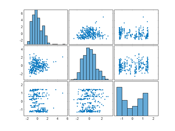
The plots can help you better understand the engineered features. For example:
The top-left plot is a histogram of the
zsc(Acceleration.*Horsepower)feature. This feature consists of the standardized element-wise product of the originalAccelerationandHorsepowerfeatures. The histogram shows thatzsc(Acceleration.*Horsepower)has a few outlying values greater than 3.The bottom-left plot is a scatter plot that compares the
zsc(Acceleration.*Horsepower)values (along the x-axis) to thezsc(Horsepower.*Weight)values (along the y-axis). The scatter plot shows that thezsc(Horsepower.*Weight)values tend to increase as thezsc(Acceleration.*Horsepower)values increase. Note that this plot contains the same information as the top-right plot, but with the axes flipped.
Create newTestTbl by applying the transformations stored in the object Transformer to the test data.
newTestTbl = transform(Transformer,testTbl);
Train an SVM regression model with a Gaussian kernel using the transformed training set newTrainTbl. Let the fitrsvm function find an appropriate scale value for the kernel function. Compute the mean squared error (MSE) of the model on the transformed test set newTestTbl.
Mdl = fitrsvm(newTrainTbl,"MPG",KernelFunction="gaussian", ...
    KernelScale="auto");
testMSE = loss(Mdl,newTestTbl,"MPG")
testMSE =
8.3955
Compare the predicted test set response values to the true response values. Plot the predicted miles per gallon (MPG) along the vertical axis and the true MPG along the horizontal axis. Points on the reference line indicate correct predictions. A good model produces predictions that are scattered near the line.
predictedTestY = predict(Mdl,newTestTbl);

plot(newTestTbl.MPG,predictedTestY,".")
hold on
plot(newTestTbl.MPG,newTestTbl.MPG)
hold off
xlabel("True Miles Per Gallon (MPG)")
ylabel("Predicted Miles Per Gallon (MPG)")

The SVM model seems to predict MPG values well.
Generate features to train a linear regression model. Compute the cross-validation mean squared error (MSE) of the model by using the crossval function.
Load the patients data set, and create a table containing the predictor data.
load patients
Tbl = table(Age,Diastolic,Gender,Height,SelfAssessedHealthStatus, ...
    Smoker,Weight);
Create a random partition for 5-fold cross-validation.
rng("default") % For reproducibility of the partition
cvp = cvpartition(size(Tbl,1),KFold=5);
Compute the cross-validation MSE for a linear regression model trained on the original features in Tbl and the Systolic response variable.
CVMdl = fitrlinear(Tbl,Systolic,CVPartition=cvp);
cvloss = kfoldLoss(CVMdl)
cvloss =
45.2990
Create the custom function myloss (shown at the end of this example). This function generates 20 features from the training data, and then applies the same training set transformations to the test data. The function then fits a linear regression model to the training data and computes the test set MSE.
Note: If you use the live script file for this example, the myloss function is already included at the end of the file. Otherwise, you need to create this function at the end of your .m file or add it as a file on the MATLAB® path.
Compute the cross-validation MSE for a linear model trained on features generated from the predictors in Tbl.
newcvloss = mean(crossval(@myloss,Tbl,Systolic,Partition=cvp))
newcvloss =
27.2205
function testloss = myloss(TrainTbl,trainY,TestTbl,testY)
[Transformer,NewTrainTbl] = genrfeatures(TrainTbl,trainY,20);
NewTestTbl = transform(Transformer,TestTbl);
Mdl = fitrlinear(NewTrainTbl,trainY);
testloss = loss(Mdl,NewTestTbl,testY);
end
Input Arguments
Name-Value Arguments
Output Arguments
Tips
By default, when
TargetLearneris"linear"or"gaussian-svm", the software generates new features from numeric predictors by using z-scores (seeTransformedDataStandardization). You can change the type of standardization for the transformed features. However, using some method of standardization, thereby avoiding the"none"specification, is strongly recommended. Fitting linear and SVM models works best with standardized data.When you generate features to create an SVM model with good predictive performance, specify
KernelScaleas"auto"in the call tofitrsvm. This specification allows the software to find an appropriate scale value for the SVM kernel function.