randomEffects
Estimates of random effects and related statistics
Syntax
Description
Examples
Load the sample data.
load carbigFit a linear mixed-effects model for miles per gallon (MPG), with fixed effects for acceleration and horsepower, and potentially correlated random effects for intercept and acceleration, grouped by the model year. First, store the data in a table.
tbl = table(Acceleration,Horsepower,Model_Year,MPG);
Fit the model.
lme = fitlme(tbl, 'MPG ~ Acceleration + Horsepower + (Acceleration|Model_Year)');Compute the BLUPs of the random-effects coefficients and display the names of the corresponding random effects.
[B,Bnames]
= randomEffects(lme)
B = 26×1

    3.1270
   -0.2426
   -1.6532
   -0.0086
    1.2075
   -0.2179
    4.4107
   -0.4887
   -1.3103
   -0.0208
    2.8029
   -0.3790
    0.0865
   -0.1280
    0.4216
      ⋮
Bnames=26×3 table
        Group         Level           Name
    ______________    ______    ________________

    {'Model_Year'}    {'70'}    {'(Intercept)' }
    {'Model_Year'}    {'70'}    {'Acceleration'}
    {'Model_Year'}    {'71'}    {'(Intercept)' }
    {'Model_Year'}    {'71'}    {'Acceleration'}
    {'Model_Year'}    {'72'}    {'(Intercept)' }
    {'Model_Year'}    {'72'}    {'Acceleration'}
    {'Model_Year'}    {'73'}    {'(Intercept)' }
    {'Model_Year'}    {'73'}    {'Acceleration'}
    {'Model_Year'}    {'74'}    {'(Intercept)' }
    {'Model_Year'}    {'74'}    {'Acceleration'}
    {'Model_Year'}    {'75'}    {'(Intercept)' }
    {'Model_Year'}    {'75'}    {'Acceleration'}
    {'Model_Year'}    {'76'}    {'(Intercept)' }
    {'Model_Year'}    {'76'}    {'Acceleration'}
    {'Model_Year'}    {'77'}    {'(Intercept)' }
    {'Model_Year'}    {'77'}    {'Acceleration'}
      ⋮
Since intercept and acceleration have potentially correlated random effects, grouped by model year of the cars, randomEffects creates a separate row for intercept and acceleration at each level of the grouping variable.
Compute the covariance parameters of the random effects.
[~,~,stats] = covarianceParameters(lme)
stats=2×1 cell array
    {3×7 classreg.regr.lmeutils.titleddataset}
    {1×5 classreg.regr.lmeutils.titleddataset}
stats{1}ans =
Covariance Type: FullCholesky
Group Name1 Name2 Type Estimate Lower Upper
Model_Year {'(Intercept)' } {'(Intercept)' } {'std' } 3.3475 1.2862 8.7119
Model_Year {'Acceleration'} {'(Intercept)' } {'corr'} -0.87971 -0.98501 -0.29676
Model_Year {'Acceleration'} {'Acceleration'} {'std' } 0.33789 0.1825 0.62558
The correlation value suggests that random effects seem negatively correlated. Plot the random effects for intercept versus acceleration to confirm this.
plot(B(1:2:end),B(2:2:end),'r*')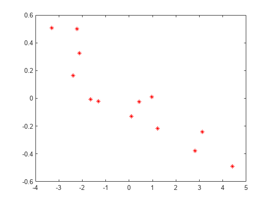
Load and display the sample data.
load fertilizer.mat
tbltbl=60×4 table
Soil Tomato Fertilizer Yield
_________ ____________ __________ _____
{'Sandy'} {'Plum' } 1 104
{'Sandy'} {'Plum' } 2 136
{'Sandy'} {'Plum' } 3 158
{'Sandy'} {'Plum' } 4 174
{'Sandy'} {'Cherry' } 1 57
{'Sandy'} {'Cherry' } 2 86
{'Sandy'} {'Cherry' } 3 89
{'Sandy'} {'Cherry' } 4 98
{'Sandy'} {'Heirloom'} 1 65
{'Sandy'} {'Heirloom'} 2 62
{'Sandy'} {'Heirloom'} 3 113
{'Sandy'} {'Heirloom'} 4 84
{'Sandy'} {'Grape' } 1 54
{'Sandy'} {'Grape' } 2 86
{'Sandy'} {'Grape' } 3 89
{'Sandy'} {'Grape' } 4 115
⋮
The table tbl contains data from a split-plot experiment, where soil is divided into three blocks based on the soil type: sandy, silty, and loamy. Each block is divided into five plots, where five different types of tomato plants (cherry, heirloom, grape, vine, and plum) are randomly assigned to these plots. The tomato plants in the plots are then divided into subplots, where each subplot is treated by one of four fertilizers. This is simulated data.
Convert Tomato, Soil, and Fertilizer to categorical variables.
tbl.Tomato = categorical(tbl.Tomato);
tbl.Soil = categorical(tbl.Soil);
tbl.Fertilizer = categorical(tbl.Fertilizer);
Fit a linear mixed-effects model, where Fertilizer and Tomato are the fixed-effects variables, and the mean yield varies by the block (soil type), and the plots within blocks (tomato types within soil types) independently.
lme = fitlme(tbl,"Yield ~ Fertilizer * Tomato + (1|Soil) + (1|Soil:Tomato)");Compute the BLUPs and related statistics for random effects.
[~,~,stats] = randomEffects(lme)
stats =
    Random effect coefficients: DFMethod = 'Residual', Alpha = 0.05

    Group                  Level                     Name                   Estimate    SEPred    tStat       DF    pValue      Lower      Upper
    {'Soil'       }        {'Loamy'         }        {'(Intercept)'}         1.0061     2.3374     0.43044    40     0.66918     -3.718     5.7303
    {'Soil'       }        {'Sandy'         }        {'(Intercept)'}        -1.5236     2.3374    -0.65181    40     0.51825    -6.2477     3.2006
    {'Soil'       }        {'Silty'         }        {'(Intercept)'}        0.51744     2.3374     0.22137    40     0.82593    -4.2067     5.2416
    {'Soil:Tomato'}        {'Loamy Cherry'  }        {'(Intercept)'}          12.46     7.1765      1.7362    40    0.090224    -2.0443     26.964
    {'Soil:Tomato'}        {'Loamy Grape'   }        {'(Intercept)'}        -2.6429     7.1765    -0.36827    40     0.71461    -17.147     11.861
    {'Soil:Tomato'}        {'Loamy Heirloom'}        {'(Intercept)'}         16.681     7.1765      2.3244    40    0.025269     2.1766     31.185
    {'Soil:Tomato'}        {'Loamy Plum'    }        {'(Intercept)'}        -5.0172     7.1765    -0.69911    40     0.48853    -19.522     9.4872
    {'Soil:Tomato'}        {'Loamy Vine'    }        {'(Intercept)'}        -4.6874     7.1765    -0.65316    40     0.51739    -19.192     9.8169
    {'Soil:Tomato'}        {'Sandy Cherry'  }        {'(Intercept)'}        -17.393     7.1765     -2.4235    40    0.019987    -31.897    -2.8882
    {'Soil:Tomato'}        {'Sandy Grape'   }        {'(Intercept)'}        -7.3679     7.1765     -1.0267    40     0.31075    -21.872     7.1364
    {'Soil:Tomato'}        {'Sandy Heirloom'}        {'(Intercept)'}         -8.621     7.1765     -1.2013    40     0.23671    -23.125     5.8833
    {'Soil:Tomato'}        {'Sandy Plum'    }        {'(Intercept)'}          7.669     7.1765      1.0686    40     0.29165    -6.8353     22.173
    {'Soil:Tomato'}        {'Sandy Vine'    }        {'(Intercept)'}        0.28246     7.1765    0.039359    40      0.9688    -14.222     14.787
    {'Soil:Tomato'}        {'Silty Cherry'  }        {'(Intercept)'}         4.9326     7.1765     0.68732    40     0.49585    -9.5718     19.437
    {'Soil:Tomato'}        {'Silty Grape'   }        {'(Intercept)'}         10.011     7.1765      1.3949    40     0.17073    -4.4935     24.515
    {'Soil:Tomato'}        {'Silty Heirloom'}        {'(Intercept)'}        -8.0599     7.1765     -1.1231    40      0.2681    -22.564     6.4444
    {'Soil:Tomato'}        {'Silty Plum'    }        {'(Intercept)'}        -2.6519     7.1765    -0.36952    40     0.71369    -17.156     11.852
    {'Soil:Tomato'}        {'Silty Vine'    }        {'(Intercept)'}          4.405     7.1765      0.6138    40     0.54282    -10.099     18.909
The first three rows contain the random-effects estimates and the statistics for the three levels, Loamy, Sandy, and Silty of the grouping variable Soil. The corresponding -values 0.66918, 0.51825, and 0.82593 indicate that these random-effects are not significantly different from 0. The following 15 rows include the BLUPS of random-effects estimates for the intercept, grouped by the variable Tomato nested in Soil, i.e. interaction of Tomato and Soil.
Load the sample data.
load shiftFit a linear mixed-effects model with a random intercept grouped by operator, to assess if there is a significant difference in the performance according to the time of the shift. Use the restricted maximum likelihood method.
lme = fitlme(shift,'QCDev ~ Shift + (1|Operator)');Compute the 99% confidence intervals for random effects using the residuals option to compute the degrees of freedom. This is the default method.
[~,~,stats] = randomEffects(lme,'Alpha',0.01)stats =
Random effect coefficients: DFMethod = 'Residual', Alpha = 0.01
Group Level Name Estimate SEPred tStat DF pValue Lower Upper
{'Operator'} {'1'} {'(Intercept)'} 0.57753 0.90378 0.63902 12 0.53482 -2.1831 3.3382
{'Operator'} {'2'} {'(Intercept)'} 1.1757 0.90378 1.3009 12 0.21772 -1.5849 3.9364
{'Operator'} {'3'} {'(Intercept)'} -2.1715 0.90378 -2.4027 12 0.033352 -4.9322 0.58909
{'Operator'} {'4'} {'(Intercept)'} 2.3655 0.90378 2.6174 12 0.022494 -0.39511 5.1261
{'Operator'} {'5'} {'(Intercept)'} -1.9472 0.90378 -2.1546 12 0.052216 -4.7079 0.81337
Compute the 99% confidence intervals for random effects using the Satterthwaite approximation to compute the degrees of freedom.
[~,~,stats] = randomEffects(lme,'DFMethod','satterthwaite','Alpha',0.01)
stats =
    Random effect coefficients: DFMethod = 'Satterthwaite', Alpha = 0.01

    Group               Level        Name                   Estimate    SEPred     tStat      DF        pValue      Lower       Upper
    {'Operator'}        {'1'}        {'(Intercept)'}        0.57753     0.90378    0.63902    6.4253      0.5449      -2.684     3.839
    {'Operator'}        {'2'}        {'(Intercept)'}         1.1757     0.90378     1.3009    6.4253     0.23799     -2.0858    4.4372
    {'Operator'}        {'3'}        {'(Intercept)'}        -2.1715     0.90378    -2.4027    6.4253    0.050386      -5.433      1.09
    {'Operator'}        {'4'}        {'(Intercept)'}         2.3655     0.90378     2.6174    6.4253    0.037302    -0.89598     5.627
    {'Operator'}        {'5'}        {'(Intercept)'}        -1.9472     0.90378    -2.1546    6.4253    0.071626     -5.2087    1.3142
The Satterthwaite method usually produces smaller values for the degrees of freedom (DF), which results in larger p-values (pValue) and larger confidence intervals (Lower and Upper) for the random-effects estimates.
Input Arguments
Name-Value Arguments
Output Arguments
Version History
Introduced in R2013b
See Also
LinearMixedModel | fitlme | coefCI | coefTest | fixedEffects