Main Content

paretotails

Piecewise distribution with Pareto tails

Description

A paretotails object is a piecewise distribution with generalized Pareto distributions (GPDs) in the tails.

A paretotails object consists of one or two GPDs in the tails and another distribution in the center. You can specify the distribution type for the center by using the cdffun argument of paretotails when you create an object. Valid values are 'ecdf', 'kernel', and a function handle.

paretotails fits a distribution of type cdffun to the observations (x) and finds the quantiles corresponding to the lower and upper tail cumulative probabilities (pl and pu, respectively). Then, paretotails fits two GPDs to the lower 100*pl percent of the observations and the upper 100*(1–pu) percent of the observations, respectively. If x does not have at least two distinct observations in a tail, then paretotails does not create the corresponding tail segment.

Use the object functions boundary, segment, upperparams, and lowerparams to find distribution characteristics. lowerparams and upperparams return the parameters of the GPDs in the tails. boundary returns the boundary points between piecewise distribution segments, segment returns the segment of a piecewise distribution containing input values, and nsegments returns the number of segments in an object.

Use the object functions cdf, icdf, pdf, and random to evaluate the distribution. These functions are well suited to copula and other Monte Carlo simulations. pdf returns the GPD density in the tails and the slope of the cumulative distribution function (cdf) in the center. These probability density function (pdf) values in the center are generally not good estimates of the underlying density of the original data.

Creation

Create a piecewise distribution object using paretotails.

Description

pd = paretotails(x,pl,pu) returns the piecewise distribution object pd, which consists of the empirical distribution in the center and generalized Pareto distributions in the tails. Specify the boundaries of the tails using the lower and upper tail cumulative probabilities pl and pu, respectively.

example

pd = paretotails(x,pl,pu,cdffun) specifies the type of center distribution segment using cdffun.

example

Input Arguments

expand all

Input data, specified as a numeric vector.

Data Types: double

Lower tail cumulative probability, specified as a numeric scalar in the range [0,1]. The quantile of pl is the boundary of the lower tail observations.

If pl is 0 or x does not have at least two distinct observations in the lower tail, then paretotails divides the input data in x into two groups, center and upper tail. In this case, the fitted piecewise distribution object pd consists of two segments: the empirical distribution in the center and GPD in the upper tail.

Example: 0.1

Data Types: single | double

Upper tail cumulative probability, specified as a numeric scalar in the range [0,1]. The quantile of pu is the boundary of the upper tail observations.

If pu is 1 or x does not have at least two distinct observations in the upper tail, then paretotails divides the input data in x into two groups, center and lower tail. In this case, the fitted piecewise distribution object pd consists of two segments: the empirical distribution in the center and GPD in the lower tail.

Example: 0.9

Data Types: single | double

Type of center distribution segment, specified as 'ecdf', 'kernel', or a function handle.

ValueDescription
'ecdf'

Interpolated empirical cdf.

paretotails uses values in x as the midpoints in the vertical steps of the empirical cdf, and computes the estimates for the points between the values in x by linear interpolation. For details about how to find the interpolated empirical cdf, see A Piecewise Linear Nonparametric CDF Estimate.

'kernel'

Interpolated kernel smoothing estimate of the cdf.

paretotails uses the ksdensity function to find cdf estimates for 100 points in the range of x, and uses linear interpolation to compute the estimates for the points between the 100 points.

'kernel' is equivalent to specifying a function handle fun = @(x)ksdensity(x,'function','cdf');.

function handle

Interpolated estimates using a specified function.

paretotails uses a handle to a function of the form [p,xi] = fun(x) that accepts the input data vector x and returns a vector p of cdf values and a vector xi of evaluation points. Values in xi must be sorted and distinct but do not have to equal the values in x. The paretotails function computes the cdf estimates for the points between the values in xi by linear interpolation.

paretotails uses cdffun to compute the quantiles corresponding to pl and pu.

Example: 'kernel'

Properties

expand all

This property is read-only.

Number of segments, including the center segment and tail segments in a paretotail object, specified as a scalar. NumSegments is 3, 2, or 1 if the number of the tail segments in the object is 2, 1, or 0, respectively.

Data Types: double

This property is read-only.

Lower tail GPD parameters, fit to the lower extreme observations in x, specified as a numeric vector. The first value is the shape parameter and the second value is the scale parameter of the GPD.

The location parameter of the lower tail GPD is equal to the quantile of pl. Use the boundary function to return the location parameter. For example, run [p,q] = boundary(pd), where pd is a paretotails object. q(1) is the location parameter.

Data Types: single | double

This property is read-only.

Upper tail GPD parameters, fit to the upper extreme observations in x, specified as a numeric vector. The first value is the shape parameter and the second value is the scale parameter of the GPD.

The location parameter of the upper tail GPD is equal to the quantile of pu. Use the boundary function to return the location parameter. For example, run [p,q] = boundary(pd), where pd is a paretotails object. q(2) is the location parameter.

Data Types: single | double

Object Functions

boundaryPiecewise distribution boundaries
cdfCumulative distribution function
icdfInverse cumulative distribution function
lowerparamsLower Pareto tail parameters
nsegmentsNumber of segments in piecewise distribution
pdfProbability density function
randomRandom numbers
segmentPiecewise distribution segments containing input values
upperparamsUpper Pareto tail parameters

Examples

collapse all

Generate a sample data set and fit a piecewise distribution with Pareto tails to the data. Specify an empirical distribution for the center by using paretotails with its default settings.

Generate a sample data set containing 100 random numbers from a t distribution with 3 degrees of freedom.

rng('default');  % For reproducibility
t = trnd(3,100,1);

Create a paretotails object by fitting a piecewise distribution to t. Specify the boundaries of the tails using the lower and upper tail cumulative probabilities so that a fitted object consists of the empirical distribution for the middle 80% of the data set and GPDs for the lower and upper 10% of the data set.

pd = paretotails(t,0.1,0.9)
pd = 
Piecewise distribution with 3 segments
      -Inf < x < -1.84875    (0 < p < 0.1): lower tail, GPD(0.183032,1.00347)
   -1.84875 < x < 2.07662  (0.1 < p < 0.9): interpolated empirical cdf
        2.07662 < x < Inf    (0.9 < p < 1): upper tail, GPD(0.333239,1.19705)

Each line of the object display shows the summary of each segment, including the GPD parameters (shape and scale parameters) and the boundary values in the quantiles and cumulative probabilities. Use the object functions boundary, lowerparams, and upperparams to return these values.

You can use the nsegments function to return the number of segments and the segment function to return the segment that contains input values.

You can also use the distribution functions cdf, icdf, pdf, and random to evaluate the distribution and generate random samples.

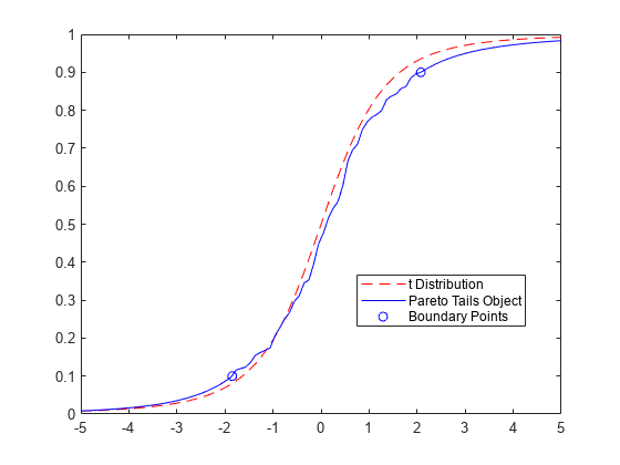
Plot the cdf of the t distribution and the cdf of the paretotails object on the same figure.

x = linspace(-5,5);
plot(x,tcdf(x,3),'r--')
hold on
plot(x,cdf(pd,x),'b-')

Find the boundary points between the segments of the paretotails object by using boundary, and mark the points on the figure.

[p,q] = boundary(pd);
plot(q,p,'bo')
legend('t Distribution','Pareto Tails Object','Boundary Points','Location','best')
hold off

Figure contains an axes object. The axes object contains 3 objects of type line. One or more of the lines displays its values using only markers These objects represent t Distribution, Pareto Tails Object, Boundary Points.

Generate a sample data set and fit a piecewise distribution with Pareto tails to the data. Fit a center segment by using paretotails with a function handle.

Generate a sample data set containing 20% outliers.

rng('default');  % For reproducibility
left_tail = -exprnd(1,100,1);
right_tail = exprnd(5,100,1);
center = randn(800,1);
x = [left_tail;center;right_tail];

Define a function handle using ksdensity to specify a nondefault value of the bandwidth.

myfun1 = @(x)ksdensity(x,'Bandwidth',.1,'Function','cdf');

Create a paretotails object by fitting a piecewise distribution with the specified kernel smoothing estimator to x. Specify the boundaries of the tails using the lower and upper tail cumulative probabilities so that a fitted object consists of the kernel estimator for the middle 80% of the data set and GPDs for the lower and upper 10% of the data set.

pd1 = paretotails(x,0.1,0.9,myfun1)
pd1 = 
Piecewise distribution with 3 segments
      -Inf < x < -1.35204    (0 < p < 0.1): lower tail, GPD(0.0104112,0.54947)
   -1.35204 < x < 1.80824  (0.1 < p < 0.9): function: @(x)ksdensity(x,'Bandwidth',.1,'Function','cdf')
        1.80824 < x < Inf    (0.9 < p < 1): upper tail, GPD(0.227542,3.10586)

You can also use a parametric distribution for the center segment. Define a function that fits a normal distribution to data and returns the cdf values, and pass the function handle when you create a paretotails object.

pd2 = paretotails(x,0.1,0.9,@myfun2)
pd2 = 
Piecewise distribution with 3 segments
      -Inf < x < -2.70875    (0 < p < 0.1): lower tail, GPD(-0.358104,0.831855)
   -2.70875 < x < 3.52195  (0.1 < p < 0.9): function: myfun2
        3.52195 < x < Inf    (0.9 < p < 1): upper tail, GPD(-0.0661815,5.04694)

function [p,xi] = myfun2(x)
    pd = fitdist(x,'Normal');
    xi = linspace(min(x),max(x),length(x)*2);
    p = cdf(pd,xi);
end

Version History

Introduced in R2007a

Go to top of page