pearspdf

Pearson probability density function

Since R2023b

Syntax

f = pearspdf(X,mu,sigma,skew,kurt)

[f,type] = pearspdf(X,mu,sigma,skew,kurt)

[f,type,coefs] = pearspdf(X,mu,sigma,skew,kurt)

Description

f = pearspdf(X,mu,sigma,skew,kurt) returns the probability density function (pdf) of the Pearson system evaluated at the values in X, using the mean mu, standard deviation sigma, skewness skew, and kurtosis kurt.

[f,type] = pearspdf(X,mu,sigma,skew,kurt) also returns the type of the specified distribution within the Pearson system.

[f,type,coefs] = pearspdf(X,mu,sigma,skew,kurt) also returns the coefficients in the denominator of the differential equation

$$\frac{p\text{'}(x)}{p(x)}=-\frac{a+(x-\mu )}{b_0+b_1(x-\mu )+b_2{(x-\mu )}^2},$$

which defines the Pearson pdf $$p(x)$$.

Examples

Compute and Plot Pearson Probability Density Function

Define the variables mu, sigma, skew, and kurtosis, which contain values for the mean, standard deviation, skewness, and kurtosis of a Pearson distribution, respectively.

mu = 0;
sigma = 2;
skew = 0;
kurtosis = 3;

A Pearson distribution with a skewness of 0 and kurtosis of 3 is equivalent to the normal distribution.

Create a vector X of points from —7 to 7 using the linspace function. Evaluate the pdf for the Pearson distribution given by mu, sigma, skew, and kurtosis at the points in X. Plot the result together with the pdf for the standard normal distribution.

X = linspace(-7,7,1000);
Fp = pearspdf(X,mu,sigma,skew,kurtosis);
Fn = normpdf(X,mu,sigma);

figure
hold on
plot(X,Fp)
plot(X,Fn)
legend(["Pearson PDF" "Normal PDF"])

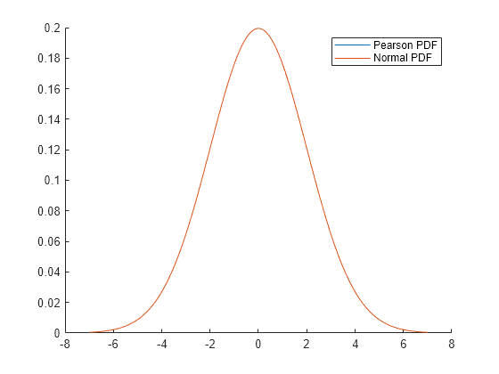
The plot shows that the blue curve for the Pearson distribution pdf is completely hidden by the red curve for the normal distribution pdf. This result indicates that the Pearson pdf is identical to the normal distribution pdf.

Compute Lower Bound for Type 6 Pearson Distribution

Define the variables mu, sigma, skew, and kurtosis, which contain values for the mean, standard deviation, skewness, and kurtosis of a Pearson distribution, respectively.

mu = 2;
sigma = 1;
skew = 2;
kurtosis = 10;

Return the type of the Pearson distribution given by mu, sigma, skew, and kurtosis, and return the coefficients of the corresponding quadratic polynomial.

[~,type,coefs] = pearspdf([],mu,sigma,skew,kurtosis)

type = 6

coefs = 1×3

    0.8235    0.7647    0.0588

The output shows that the distribution is of type 6, and displays the coefficients for the quadratic polynomial. Type 6 Pearson distributions are bounded on one side. The bound is calculated from the roots of the quadratic polynomial in the denominator of the differential equation that defines the pdf. For more information, see Probability Density Function and Support.

Find the roots of the quadratic polynomial by using the fliplr function to reverse the order of the coefficients in coefs. Pass the result to the roots function.

coefs = fliplr(coefs);
a = roots(coefs)

a = 2×1

  -11.8151
   -1.1849

Both of the roots are negative. This result indicates that the distribution has a lower bound, which you can calculate by using mu, sigma, and the largest root in a.

Calculate the lower bound for the distribution.

lower = sigma*max(a) + mu;

Create a vector of points from lower to 10 by using the linspace function.

X = linspace(lower,10,1000);

Evaluate the pdf for the distribution at the points in X, and then plot the result.

F = pearspdf(X,mu,sigma,skew,kurtosis);
plot(X,F)
hold on
xlim([lower,10])

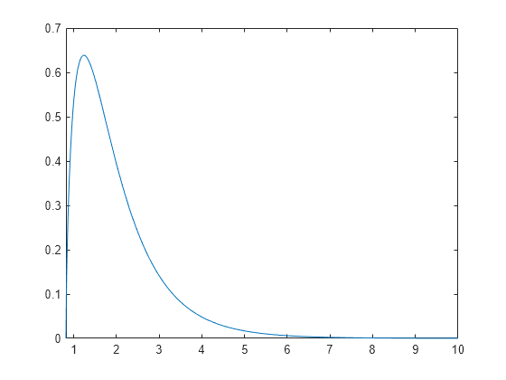
The distribution pdf has a shape typical of an F-distribution.

Input Arguments

X — Values at which to evaluate Pearson pdf

scalar | numeric array

Values at which to evaluate the Pearson pdf, specified as a scalar or a numeric array.

To evaluate the pdf at multiple values, specify X using an array. To evaluate the pdfs of multiple distributions, specify either mu or sigma (or both) using arrays. If one or more of the input arguments X, mu, and sigma are arrays, then the array sizes must be the same. In this case, pearspdf expands each scalar input into a constant array of the same size as the array inputs. Each element in f is the pdf value of the distribution specified by the corresponding elements in mu and sigma, evaluated at the corresponding element in X.

Example: [0 0.4 0.8 0.12]

Data Types: single | double

mu — Mean

scalar | numeric array

Mean of the Pearson distribution, specified as a scalar or a numeric array.

To evaluate the pdf at multiple values, specify X using an array. To evaluate the pdfs of multiple distributions, specify either mu or sigma (or both) using arrays. If one or more of the input arguments X, mu, and sigma are arrays, then the array sizes must be the same. In this case, pearspdf expands each scalar input into a constant array of the same size as the array inputs. Each element in f is the pdf value of the distribution specified by the corresponding elements in mu and sigma, evaluated at the corresponding element in X.

Example: [0 1 2; 0 1 2]

Data Types: single | double

sigma — Standard deviation

positive scalar | array of positive values

Standard deviation of the Pearson distribution, specified as a positive scalar or an array of positive values.

To evaluate the pdf at multiple values, specify X using an array. To evaluate the pdfs of multiple distributions, specify either mu or sigma (or both) using arrays. If one or more of the input arguments X, mu, and sigma are arrays, then the array sizes must be the same. In this case, pearspdf expands each scalar input into a constant array of the same size as the array inputs. Each element in f is the pdf value of the distribution specified by the corresponding elements in mu and sigma, evaluated at the corresponding element in X.

Example: [1 1 1; 2 2 2]

Data Types: single | double

skew — Skewness

scalar

Skewness for the Pearson distribution, specified as a scalar. The value of skew must be less than sqrt(kurt - 1). For more information, see Skewness.

Example: 3

Data Types: single | double

kurt — Kurtosis

scalar

Kurtosis for the Pearson distribution, specified as a scalar. The value of kurt must be greater than skew^2 + 1. For more information, see Kurtosis.

Example: 11

Data Types: single | double

Output Arguments

f — Pearson pdf

scalar | numeric array

Pearson pdf evaluated at the values in X, returned as a scalar or a numeric array. f is the same size as X, mu, and sigma after any necessary scalar expansion. Each element in f is the pdf value of the distribution specified by skew, kurt, and the corresponding elements in mu and sigma, evaluated at the corresponding value in X.

type — Type of Pearson distribution

integer from interval [0 7] | NaN

Type of Pearson distribution used to calculate the pdf, returned as an integer from the interval [0 7] or NaN. If the distribution parameters are invalid, pearspdf returns NaN.

This table describes the distribution corresponding to each Pearson distribution type.

Pearson Distribution Type	Description
0	Normal
1	4-parameter beta
2	Symmetric 4-parameter beta
3	3-parameter gamma
4	Distribution specific to the Pearson system with pdf proportional to $${\left(1+{\left(\frac{x-\mu }{\sigma }\right)}^2\right)}^{-a}\exp (-b\arctan (\frac{x-\mu }{\sigma }))$$, where a and b are quantities related to the differential equation that defines the Pearson distribution
5	Inverse 3-parameter gamma
6	F location scale
7	Student's t location scale

coefs — Quadratic polynomial coefficients

numeric 1-by-3 vector

Quadratic polynomial coefficients, returned as a numeric 1-by-3 vector. The ith element of coefs is the coefficient $$b_i$$ in the differential equation

$$\frac{p\text{'}(x)}{p(x)}=-\frac{a+(x-\mu )}{b_0+b_1(x-\mu )+b_2{(x-\mu )}^2},$$

which defines the Pearson distribution pdf $$p(x)$$.

You can calculate the support for the Pearson distribution pdf using coefs. For more information, see Probability Density Function and Support.

More About

Skewness

Skewness is a measure of the asymmetry of the data around the sample mean. If skewness is negative, the data spreads out more to the left of the mean than to the right. If skewness is positive, the data spreads out more to the right. The skewness of the normal distribution (or any perfectly symmetric distribution) is zero.

The skewness of a distribution is defined as

$$s=\frac{E{\left(x-\mu \right)}^3}{{\sigma }^3},$$

where µ is the mean of x, σ is the standard deviation of x, and E(t) represents the expected value of the quantity t.

Kurtosis

Kurtosis is a measure of how prone a distribution is to outliers. The kurtosis of the normal distribution is 3. Distributions that are more prone to outliers than the normal distribution have a kurtosis value greater than 3; distributions that are less prone have a kurtosis value less than 3. Some definitions of kurtosis subtract 3 from the computed value, so that the normal distribution has a kurtosis of 0. pearspdf does not use this convention.

The kurtosis of a distribution is defined as

$$k=\frac{E{(x-\mu )}^4}{{\sigma }^4},$$

where μ is the mean of x, σ is the standard deviation of x, and E(t) represents the expected value of the quantity t.

Alternative Functionality

pearspdf is a function specific to the Pearson distribution. Statistics and Machine Learning Toolbox™ also offers the generic function pdf, which supports various probability distributions. To use pdf, specify the probability distribution name and its parameters.

References

[1] Johnson, Norman Lloyd, et al. "Continuous Univariate Distributions." 2nd ed, vol. 1, Wiley, 1994.

[2] Willink, R. "A Closed-Form Expression for the Pearson Type IV Distribution Function." Australian & New Zealand Journal of Statistics, vol. 50, no. 2, June 2008, pp. 199–205. https://onlinelibrary.wiley.com/doi/10.1111/j.1467-842X.2008.00508.x.

Extended Capabilities

GPU Arrays

Accelerate code by running on a graphics processing unit (GPU) using Parallel Computing Toolbox™.

This function fully supports GPU arrays. For more information, see Run MATLAB Functions on a GPU (Parallel Computing Toolbox).

Version History

Introduced in R2023b