Poisson Distribution
Overview
The Poisson distribution is a one-parameter family of curves that models the number of times a random event occurs. This distribution is appropriate for applications that involve counting the number of times a random event occurs in a given amount of time, distance, area, and so on. Sample applications that involve Poisson distributions include the number of Geiger counter clicks per second, the number of people walking into a store in an hour, and the number of packets lost over a network per minute.
Statistics and Machine Learning Toolbox™ offers several ways to work with the Poisson distribution.
Create a probability distribution object
PoissonDistributionby fitting a probability distribution to sample data or by specifying parameter values. Then, use object functions to evaluate the distribution, generate random numbers, and so on.Work with the Poisson distribution interactively by using the Distribution Fitter app. You can export an object from the app and use the object functions.
Use distribution-specific functions (
poisscdf,poisspdf,poissinv,poisstat,poissfit,poissrnd) with specified distribution parameters. The distribution-specific functions can accept parameters of multiple Poisson distributions.Use generic distribution functions (
cdf,icdf,pdf,random) with a specified distribution name ('Poisson') and parameters.
Parameters
The Poisson distribution uses the following parameter.
| Parameter | Description | Support |
|---|---|---|
lambda (λ) | Mean |
The parameter λ is also equal to the variance of the Poisson distribution.
The sum of two Poisson random variables with parameters λ1 and λ2 is a Poisson random variable with parameter λ = λ1 + λ2 .
Probability Density Function
The probability density function (pdf) of the Poisson distribution is
The result is the probability of exactly x occurrences of the random event. For discrete distributions, the pdf is also known as the probability mass function (pmf).
For an example, see Compute Poisson Distribution pdf.
Cumulative Distribution Function
The cumulative distribution function (cdf) of the Poisson distribution for x ≥ 0 is
The result is the probability of at most x occurrences of the random event.
For an example, see Compute Poisson Distribution cdf.
Examples
Compute Poisson Distribution pdf
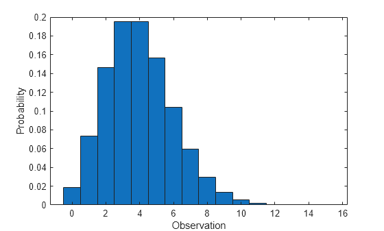
Compute the pdf of the Poisson distribution with parameter lambda = 4.
x = 0:15;
y = poisspdf(x,4);
Plot the pdf with bars of width 1.
figure
bar(x,y,1)
xlabel('Observation')
ylabel('Probability')

Compute Poisson Distribution cdf
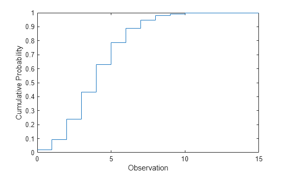
Compute the cdf of the Poisson distribution with parameter lambda = 4.
x = 0:15;
y = poisscdf(x,4);
Plot the cdf.
figure
stairs(x,y)
xlabel('Observation')
ylabel('Cumulative Probability')

Compare Poisson and Normal Distribution pdfs
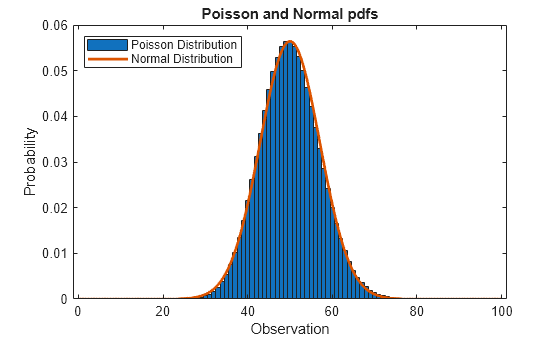
When lambda is large, the Poisson distribution can be approximated by the normal distribution with mean lambda and variance lambda.
Compute the pdf of the Poisson distribution with parameter lambda = 50.
lambda = 50;
x1 = 0:100;
y1 = poisspdf(x1,lambda);
Compute the pdf of the corresponding normal distribution.
mu = lambda;
sigma = sqrt(lambda);
x2 = 0:0.1:100;
y2 = normpdf(x2,mu,sigma);
Plot the pdfs on the same axis.
figure
bar(x1,y1,1)
hold on
plot(x2,y2,'LineWidth',2)
xlabel('Observation')
ylabel('Probability')
title('Poisson and Normal pdfs')
legend('Poisson Distribution','Normal Distribution','location','northwest')
hold off

The pdf of the normal distribution closely approximates the pdf of the Poisson distribution.
Related Distributions
Binomial Distribution — The binomial distribution is a two-parameter discrete distribution that counts the number of successes in N independent trials with the probability of success p. The Poisson distribution is the limiting case of a binomial distribution where N approaches infinity and p goes to zero while Np = λ. See Compare Binomial and Poisson Distribution pdfs.
Exponential Distribution — The exponential distribution is a one-parameter continuous distribution that has parameter μ (mean). The Poisson distribution models counts of the number of times a random event occurs in a given amount of time. In such a model, the amount of time between occurrences is modeled by the exponential distribution with mean .
Normal Distribution — The normal distribution is a two-parameter continuous distribution that has parameters μ (mean) and σ (standard deviation). When λ is large, the Poisson distribution can be approximated by the normal distribution with μ = λ and σ2 = λ. See Compare Poisson and Normal Distribution pdfs.
References
[1] Abramowitz, Milton, and Irene A. Stegun, eds. Handbook of Mathematical Functions: With Formulas, Graphs, and Mathematical Tables. 9. Dover print.; [Nachdr. der Ausg. von 1972]. Dover Books on Mathematics. New York, NY: Dover Publ, 2013.
[2] Devroye, Luc. Non-Uniform Random Variate Generation. New York, NY: Springer New York, 1986. https://doi.org/10.1007/978-1-4613-8643-8
[3] Evans, Merran, Nicholas Hastings, and Brian Peacock. Statistical Distributions. 2nd ed. New York: J. Wiley, 1993.
[4] Loader, Catherine. Fast and Accurate Computation of Binomial Probabilities. July 9, 2000.
See Also
PoissonDistribution | poisscdf | poisspdf | poissinv | poisstat | poissfit | poissrnd