plot
Description
plot( creates a horizontal bar graph
using the Shapley values of the explainer)shapley object
explainer.
If
explainercontains one query point only, then the bar graph displays Shapley values. These values are stored in theShapleyproperty of the object. Each bar shows the Shapley value of each feature (predictor) in the blackbox model (explainer.) for the query point (BlackboxModelexplainer.).QueryPointsIf
explainercontains multiple query points, then the bar graph displays mean absolute Shapley values. These values are stored in theMeanAbsoluteShapleyproperty of the object. For each predictor (and each class whenexplainer.BlackboxModelis a classification model), the mean absolute Shapley value is the absolute value of the Shapley values, averaged across all query points inexplainer.QueryPoints. (since R2024a)
plot(
specifies additional options using one or more name-value arguments. For example, specify
explainer,Name=Value)NumImportantPredictors=5 to plot the Shapley values of the five
features with the greatest absolute Shapley values (for one query point) or the greatest
mean absolute Shapley values (for multiple query points).
plot( displays the plot in the
target axes ax,___)ax. Specify ax as the first argument
in any of the previous syntaxes. (since R2023b)
b = plot(___)Bar object or an array of Bar objects using any of the
input argument combinations in the previous syntaxes. Use b to query or
modify the properties (Bar Properties) of an object after you create
it.
Examples
Train a classification model and create a shapley object. Then plot the Shapley values by using the object function plot.
Load the CreditRating_Historical data set. The data set contains customer IDs and their financial ratios, industry labels, and credit ratings.
tbl = readtable("CreditRating_Historical.dat");Display the first three rows of the table.
head(tbl,3)
     ID      WC_TA    RE_TA    EBIT_TA    MVE_BVTD    S_TA     Industry    Rating
    _____    _____    _____    _______    ________    _____    ________    ______

    62394    0.013    0.104     0.036      0.447      0.142       3        {'BB'}
    48608    0.232    0.335     0.062      1.969      0.281       8        {'A' }
    42444    0.311    0.367     0.074      1.935      0.366       1        {'A' }
Train a blackbox model of credit ratings by using the fitcecoc function. Use the variables from the second through seventh columns in tbl as the predictor variables. A recommended practice is to specify the class names to set the order of the classes.
blackbox = fitcecoc(tbl,"Rating", ...
    PredictorNames=tbl.Properties.VariableNames(2:7), ...
    CategoricalPredictors="Industry", ...
    ClassNames={'AAA','AA','A','BBB','BB','B','CCC'});
Create a shapley object that explains the prediction for the last observation. For faster computation, shapley subsamples 100 observations from the predictor data in tbl to compute the Shapley values.
queryPoint = tbl(end,:)
queryPoint=1×8 table
     ID      WC_TA    RE_TA    EBIT_TA    MVE_BVTD    S_TA    Industry    Rating
    _____    _____    _____    _______    ________    ____    ________    ______

    73104    0.239    0.463     0.065      2.924      0.34       2        {'AA'}
explainer = shapley(blackbox,tbl,QueryPoints=queryPoint);
For a classification model, shapley computes Shapley values using the predicted class score for each class. Display the values in the Shapley property.
explainer.Shapley
ans=6×8 table
    Predictor        AAA           AA            A            BBB            BB             B            CCC
    __________    _________    __________    __________    __________    ___________    __________    __________

    "WC_TA"        0.061172      0.023988     0.0085073    -0.0019268       -0.03895     -0.056012     -0.051658
    "RE_TA"         0.16878      0.089521      0.048741     -0.021252       -0.10389      -0.22968      -0.30796
    "EBIT_TA"     0.0013159    0.00051165    0.00039115    1.1425e-05    -0.00090913    -0.0016812    -0.0014235
    "MVE_BVTD"        1.351         1.271       0.51796      -0.27612       -0.86555       -1.0915       -0.8458
    "S_TA"        -0.012304    -0.0083217    0.00019836    -0.0026384     -2.257e-05     0.0017866    -0.0026664
    "Industry"     -0.11427     -0.053759     0.0058104      0.090519        0.11176       0.13811       0.18671
The Shapley property contains the Shapley values of all features for each class.
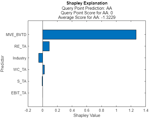
Plot the Shapley values for the predicted class by using the plot function.
plot(explainer)

The horizontal bar graph shows the Shapley values for all variables, sorted by their absolute values. Each Shapley value explains the deviation of the score for the query point from the average score of the predicted class, due to the corresponding variable.
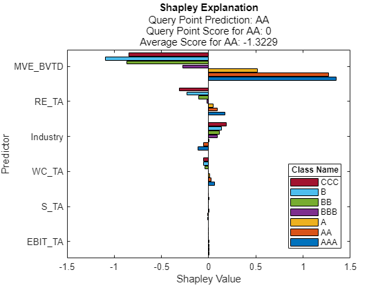
Plot the Shapley values for all classes by specifying all class names in explainer.BlackboxModel.
plot(explainer,ClassNames=explainer.BlackboxModel.ClassNames)

Train a regression model and create a shapley object. Use the object function fit to compute the Shapley values for the specified query point. Then plot the Shapley values of the predictors by using the object function plot. Specify the number of important predictors to plot when you call the plot function.
Load the carbig data set, which contains measurements of cars made in the 1970s and early 1980s.
load carbigCreate a table containing the predictor variables Acceleration, Cylinders, and so on, as well as the response variable MPG.
tbl = table(Acceleration,Cylinders,Displacement, ...
    Horsepower,Model_Year,Weight,MPG);
Removing missing values in a training set can help reduce memory consumption and speed up training for the fitrkernel function. Remove missing values in tbl.
tbl = rmmissing(tbl);
Train a blackbox model of MPG by using the fitrkernel function. Specify the Cylinders and Model_Year variables as categorical predictors. Standardize the remaining predictors.
rng("default") % For reproducibility
mdl = fitrkernel(tbl,"MPG",CategoricalPredictors=[2 5], ...
    Standardize=true);
Create a shapley object. Because mdl does not contain training data, specify the data set tbl.
explainer = shapley(mdl,tbl)
explainer =
            BlackboxModel: [1×1 RegressionKernel]
              QueryPoints: []
           BlackboxFitted: []
                  Shapley: []
                        X: [392×7 table]
    CategoricalPredictors: [2 5]
                   Method: "interventional-kernel"
                Intercept: 23.2474
               NumSubsets: 64
explainer stores the training data tbl in the X property. By default, shapley subsamples 100 observations from the data in X, and stores their indices in the SampledObservationIndices property.
Compute the Shapley values of all predictor variables for the first observation in tbl. To speed up computations, the fit object function uses the sampled observations instead of all of X to compute the Shapley values.
queryPoint = tbl(1,:)
queryPoint=1×7 table
    Acceleration    Cylinders    Displacement    Horsepower    Model_Year    Weight    MPG
    ____________    _________    ____________    __________    __________    ______    ___

         12             8            307            130            70         3504     18
explainer = fit(explainer,queryPoint);
For a regression model, fit computes Shapley values using the predicted response, and stores them in the Shapley property of the shapley object. Display the values in the Shapley property.
explainer.Shapley
ans=6×2 table
      Predictor        Value
    ______________    ________

    "Acceleration"    -0.33821
    "Cylinders"       -0.97631
    "Displacement"     -1.1425
    "Horsepower"      -0.62927
    "Model_Year"      -0.17268
    "Weight"          -0.87595
Plot the Shapley values for the query point by using the plot function. Specify to plot only the five most important predictors for the predicted response.
plot(explainer,NumImportantPredictors=5)

The horizontal bar graph shows the Shapley values for the five most important predictors, sorted by their absolute values. Each Shapley value explains the deviation of the prediction for the query point from the average, due to the corresponding variable.
Train a classification model and create a shapley object. Plot the mean absolute Shapley values for multiple query points by using the plot object function. Then plot the Shapley values for one of the query points.
Load the CreditRating_Historical data set. The data set contains customer IDs and their financial ratios, industry labels, and credit ratings.
tbl = readtable("CreditRating_Historical.dat");Display the first three rows of the table.
head(tbl,3)
     ID      WC_TA    RE_TA    EBIT_TA    MVE_BVTD    S_TA     Industry    Rating
    _____    _____    _____    _______    ________    _____    ________    ______

    62394    0.013    0.104     0.036      0.447      0.142       3        {'BB'}
    48608    0.232    0.335     0.062      1.969      0.281       8        {'A' }
    42444    0.311    0.367     0.074      1.935      0.366       1        {'A' }
Train a blackbox model of credit ratings by using the fitcecoc function. Use the variables from the second through seventh columns in tbl as the predictor variables. A recommended practice is to specify the class names to set the order of the classes.
blackbox = fitcecoc(tbl,"Rating", ...
    PredictorNames=tbl.Properties.VariableNames(2:7), ...
    CategoricalPredictors="Industry", ...
    ClassNames={'AAA','AA','A','BBB','BB','B','CCC'});
Create a shapley object that explains the predictions for multiple query points. For faster computation, shapley subsamples 100 observations from the predictor data in blackbox to compute the Shapley values. Specify the sampled observations as the query points in the call to the fit object function.
rng("default") % For reproducibility
explainer = shapley(blackbox);
queryPoints = explainer.X(explainer.SampledObservationIndices,:);
explainer = fit(explainer,queryPoints);
For a classification model, the fit function computes Shapley values using the predicted class score for each class. When you specify multiple query points, the function computes the mean absolute Shapley value for each predictor and each class, across all query points.
explainer.MeanAbsoluteShapley
ans=6×8 table
    Predictor        AAA           AA            A           BBB          BB            B           CCC
    __________    _________    __________    _________    _________    _________    _________    _________

    "WC_TA"        0.055977      0.034453     0.027338     0.023902     0.036098     0.054763     0.054931
    "RE_TA"         0.12468       0.10314      0.10787     0.087013     0.090298      0.17123       0.2552
    "EBIT_TA"     0.0015598    0.00095166    0.0011936    0.0010499    0.0010047    0.0018817    0.0017712
    "MVE_BVTD"      0.84966       0.68785      0.66198      0.94501       1.3672       1.5715       1.2161
    "S_TA"         0.025009     0.0095605     0.010606     0.014469    0.0017235    0.0075275     0.012529
    "Industry"     0.076169      0.085926     0.063854     0.046528     0.053801      0.11261      0.11829
For example, the explainer.MeanAbsoluteShapley.AAA(1) value is the average of the absolute Shapley values for the WC_TA predictor and the AAA class, across all observations in queryPoints.
explainer.MeanAbsoluteShapley.AAA(1)
ans =
0.0560
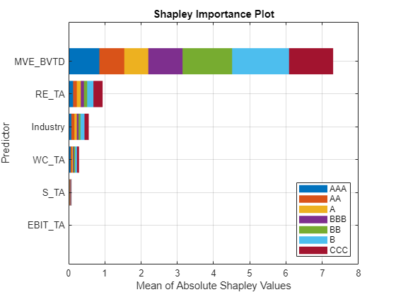
Plot the mean absolute Shapley values by using the plot object function.
plot(explainer)

For each class, the MVE_BVTD predictor has the greatest mean absolute Shapley value.
Select the first query point and determine the class prediction for the query point.
queryPoint = explainer.QueryPoints(1,:)
queryPoint=1×6 table
    WC_TA    RE_TA    EBIT_TA    MVE_BVTD    S_TA     Industry
    _____    _____    _______    ________    _____    ________

    0.197    0.471     0.067      2.304      0.602       1
queryPointPrediction = explainer.BlackboxFitted(1)
queryPointPrediction = 1×1 cell array
    {'A'}
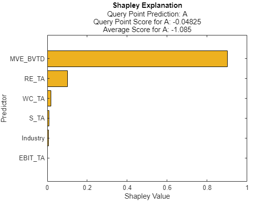
Plot the Shapley values for the query point by using the QueryPointIndices name-value argument. Change the color of the bars to match the color of the query point predicted class (A).
b = plot(explainer,QueryPointIndices=1);
b.FaceColor = [0.9290 0.6940 0.1250];

For this query point, the MVE_BVTD predictor explains the largest deviation of the class A predicted score from the average.
Input Arguments
Object explaining the blackbox model, specified as a shapley
object. explainer must contain Shapley values; that is,
explainer.Shapley must be nonempty.
Since R2023b
Axes for the plot, specified as an Axes object. If you do not
specify ax, then plot creates the plot
using the current axes. For more information on creating an Axes
object, see axes.
Name-Value Arguments
Specify optional pairs of arguments as
Name1=Value1,...,NameN=ValueN, where Name is
the argument name and Value is the corresponding value.
Name-value arguments must appear after other arguments, but the order of the
pairs does not matter.
Example: plot(explainer,NumImportantPredictors=5,ClassNames=["AAA","AA","A"])
creates a bar graph containing the Shapley values or mean absolute Shapley values of the
five most important predictors for classes AAA, AA,
and A.
Number of important predictors to plot, specified as a positive integer. The
plot function plots values for the specified number of
predictors with the greatest absolute Shapley values (for one query point) or the
greatest mean absolute Shapley values (for multiple query points).
Example: NumImportantPredictors=5 specifies to plot the five
most important predictors. The plot function determines the order
of importance by using the absolute Shapley values (for one query point) or the mean
absolute Shapley values (for multiple query points).
Data Types: single | double
Class labels to plot, specified as a numeric vector, logical vector, character
array, string array, or cell array of character vectors. The values and data types in
the ClassNames value must match those of the class names in the
ClassNames property of the machine learning model in
explainer
(explainer.BlackboxModel.ClassNames). Note that the software
accepts string arrays, cell array of character vectors, and categorical arrays
interchangeably.
You can specify one or more labels. If you specify multiple class labels, the function uses color to differentiate the classes.
The default ClassNames value depends on the number of query points.
If
explainercontains one query point, then the default value is the predicted class for the query point (theBlackboxFittedproperty ofexplainer).If
explainercontains multiple query points, then the default value is the first class in theClassNamesproperty of the machine learning model inexplainer.
This argument is valid only when the machine learning model (BlackboxModel) in explainer is a classification
model.
Example: ClassNames={'red','blue'}
Example: ClassNames=explainer.BlackboxModel.ClassNames specifies
ClassNames as all classes in
BlackboxModel.
Data Types: single | double | logical | char | string | cell | categorical
Since R2024a
Indices of the query points to use for plotting, specified as a positive integer vector.
If the
QueryPointIndicesvalue is a vectoridx, then theplotfunction returns a bar graph of the mean absolute Shapley values, averaged across the specified query points (explainer.QueryPoints(idx)).If the
QueryPointIndicesvalue is a scalar, then theplotfunction returns a bar graph of the Shapley values for the specified query point.
This argument is valid only when explainer contains multiple
query points.
Example: QueryPointIndices=1:100
Example: QueryPointIndices=50
Data Types: single | double
More About
In game theory, the Shapley value of a player is the average marginal contribution of the player in a cooperative game. In the context of machine learning prediction, the Shapley value of a feature for a query point explains the contribution of the feature to a prediction (response for regression or score of each class for classification) at the specified query point.
The Shapley value of a feature for a query point is the contribution of the feature to the deviation from the average prediction. For a query point, the sum of the Shapley values for all features corresponds to the total deviation of the prediction from the average. That is, the sum of the average prediction and the Shapley values for all features corresponds to the prediction for the query point.
For more details, see Shapley Values for Machine Learning Model.
References
[1] Lundberg, Scott M., and S. Lee. "A Unified Approach to Interpreting Model Predictions." Advances in Neural Information Processing Systems 30 (2017): 4765–774.
[2] Aas, Kjersti, Martin Jullum, and Anders Løland. "Explaining Individual Predictions When Features Are Dependent: More Accurate Approximations to Shapley Values." Artificial Intelligence 298 (September 2021).
[3] Lundberg, Scott M., G. Erion, H. Chen, et al. "From Local Explanations to Global Understanding with Explainable AI for Trees." Nature Machine Intelligence 2 (January 2020): 56–67.
Version History
Introduced in R2021aWhen the plot contains up to 12 colors, the plot function uses the
gem12 color palette in light mode and the glow12
color palette in dark mode. When the plot contains more than 12 colors, the function uses
the hsv colormap. For more information on color palettes for visualizing
multiple data series, see orderedcolors.
You can now plot mean absolute Shapley values when you compute Shapley values for
multiple query points. In the call to shapley or
fit, specify
multiple query points, and then use plot to visualize the results. You
can also specify the new QueryPointIndices name-value argument of the
plot function to plot values for a subset of the query points.
You can now specify target axes for the plot object function.
Specify an Axes object as the first input argument of the function.
When you return the Shapley values in a figure object b, the
plot function sets the TickLabelInterpreter value
of the axes to 'none' by default. That is,
b.CurrentAxes.TickLabelInterpreter is 'none'. In
previous releases, the TickLabelInterpreter value of the axes was
'tex' by default. For more information on the difference between the
'none' and 'tex' values, see TickLabelInterpreter.
MATLAB Command
You clicked a link that corresponds to this MATLAB command:
Run the command by entering it in the MATLAB Command Window. Web browsers do not support MATLAB commands.
Select a Web Site
Choose a web site to get translated content where available and see local events and offers. Based on your location, we recommend that you select: .
You can also select a web site from the following list
How to Get Best Site Performance
Select the China site (in Chinese or English) for best site performance. Other MathWorks country sites are not optimized for visits from your location.
Americas
- América Latina (Español)
- Canada (English)
- United States (English)
Europe
- Belgium (English)
- Denmark (English)
- Deutschland (Deutsch)
- España (Español)
- Finland (English)
- France (Français)
- Ireland (English)
- Italia (Italiano)
- Luxembourg (English)
- Netherlands (English)
- Norway (English)
- Österreich (Deutsch)
- Portugal (English)
- Sweden (English)
- Switzerland
- United Kingdom (English)