Apply Operators and Functions to Expressions with Units

Perform Arithmetic Operations with Units

You can perform calculations on expressions with units by using arithmetic operators, such as plus (+), minus (-), mtimes (*), and mrdivide (/). This example shows how to perform arithmetic operations on physical quantities with units and convert between different unit systems.

Load units by using symunit.

u = symunit;

Specify a physical quantity by multiplying a numeric value by a unit. For example, specify a speed of 5 meters per second.

v0_mps = 5*u.m/u.s

v0_mps = 
$$5\hspace{0.17em}\frac{\mathrm{m}\mathrm{"meter\; -\; a\; physical\; unit\; of\; length."}}{\mathrm{s}\mathrm{"second\; -\; a\; physical\; unit\; of\; time."}}$$

Add quantities that use different units. For example, add v0_mps and a speed given by v kilometers per hour.

syms v
vTotal = v0_mps + v*u.km/u.h

vTotal = 
$$5\hspace{0.17em}\frac{\mathrm{m}\mathrm{"meter\; -\; a\; physical\; unit\; of\; length."}}{\mathrm{s}\mathrm{"second\; -\; a\; physical\; unit\; of\; time."}}+v\hspace{0.17em}\frac{\mathrm{km}\mathrm{"kilometer\; -\; a\; physical\; unit\; of\; length."}}{\mathrm{h}\mathrm{"hour\; -\; a\; physical\; unit\; of\; time."}}$$

Combine and simplify unit expressions by using simplify. The simplify function selects a consistent unit system for the result. For example, simplify the total speed vTotal.

vTotal = simplify(vTotal)

vTotal = 
$$\left(1000\hspace{0.17em}v+18000\right)\hspace{0.17em}\frac{\mathrm{m}\mathrm{"meter\; -\; a\; physical\; unit\; of\; length."}}{\mathrm{h}\mathrm{"hour\; -\; a\; physical\; unit\; of\; time."}}$$

Convert the expression to another unit by using unitConvert. For example, convert the result to meters per second.

vTotal_mps = unitConvert(vTotal,u.m/u.s)

vTotal_mps = 
$$\left(\frac{5\hspace{0.17em}v}{18}+5\right)\hspace{0.17em}\frac{\mathrm{m}\mathrm{"meter\; -\; a\; physical\; unit\; of\; length."}}{\mathrm{s}\mathrm{"second\; -\; a\; physical\; unit\; of\; time."}}$$

Perform Relational Operations with Units

You can compare expressions with units by using relational operators, such as eq (==), gt (>), lt (<), ge (>=), and le (<=). This example shows how to use relational operators with symbolic units in the context of verifying physical constraints of a projectile and calculating its maximum height.

Model the height of 1-D projectile motion without air resistance. First, define the projectile's initial vertical speed as 10 kilometers per hour, the gravitational acceleration as 9.81 meters per second squared, and the time variable as an unknown value in seconds. To reflect the physical context, assume the dimensionless time variable t is always positive.

u = symunit;
syms t positive
v0_kph = 10*u.km/u.h;
g_mps2 = 9.81*u.m/u.s^2;
t_s = t*u.s;

Define the height of the projectile as a function of time.

h(t) = v0_kph*t_s - 1/2*g_mps2*t_s^2

h(t) = 
$$10\hspace{0.17em}t\hspace{0.17em}\frac{\mathrm{km}\mathrm{"kilometer\; -\; a\; physical\; unit\; of\; length."}\hspace{0.17em}\mathrm{s}\mathrm{"second\; -\; a\; physical\; unit\; of\; time."}}{\mathrm{h}\mathrm{"hour\; -\; a\; physical\; unit\; of\; time."}}-\frac{981\hspace{0.17em}{t}^2}{200}\hspace{0.17em}\mathrm{m}\mathrm{"meter\; -\; a\; physical\; unit\; of\; length."}$$

To check whether the height of this projectile is always below 1 meter, define an inequality using the relational operator <.

ineq = h(t) < 1*u.m

ineq = 
$$10\hspace{0.17em}t\hspace{0.17em}\frac{\mathrm{km}\mathrm{"kilometer\; -\; a\; physical\; unit\; of\; length."}\hspace{0.17em}\mathrm{s}\mathrm{"second\; -\; a\; physical\; unit\; of\; time."}}{\mathrm{h}\mathrm{"hour\; -\; a\; physical\; unit\; of\; time."}}-\frac{981\hspace{0.17em}{t}^2}{200}\hspace{0.17em}\mathrm{m}\mathrm{"meter\; -\; a\; physical\; unit\; of\; length."}<\mathrm{m}\mathrm{"meter\; -\; a\; physical\; unit\; of\; length."}$$

Determine whether the inequality is true for all allowed values of t by using isAlways. The result is a logical 1 (true), meaning that the height of the projectile is always below 1 meter.

tf = isAlways(ineq)

tf = logical
   1

Next, find the maximum height of this projectile. The time to reach the maximum height occurs at $t=v_0/g$, so you can substitute this value for t, taking into account all the units involved in the calculation.

hmax = subs(h(t),t,(v0_kph/g_mps2)/u.s)

hmax = 
$$\frac{5000}{981}\hspace{0.17em}\frac{{\mathrm{km}\mathrm{"kilometer\; -\; a\; physical\; unit\; of\; length."}}^2\hspace{0.17em}{\mathrm{s}\mathrm{"second\; -\; a\; physical\; unit\; of\; time."}}^2}{{\mathrm{h}\mathrm{"hour\; -\; a\; physical\; unit\; of\; time."}}^2\hspace{0.17em}\mathrm{m}\mathrm{"meter\; -\; a\; physical\; unit\; of\; length."}}$$

The result is in mixed units because unit expressions are not automatically simplified. Use simplify to combine and simplify unit expressions. Then, use vpa to convert the result to a decimal number with 32 significant digits. The maximum height is about 0.39 meter, which confirms that the height is always below 1 meter.

hmax = vpa(simplify(hmax))

hmax = $$0.39327468821182718566340720605077\hspace{0.17em}\mathrm{m}\mathrm{"meter\; -\; a\; physical\; unit\; of\; length."}$$

Call Trigonometric Functions with Units

You can apply trigonometric functions, such as sin, cos, and tan, to expressions containing angular units. This example shows how to model and plot the parabolic trajectory of a 2-D projectile using symbolic units and trigonometric functions.

Model the parabolic trajectory of 2-D projectile motion. First, define the initial speed as 20 kilometers per hour, the gravitational acceleration as 9.81 meters per second squared, the dimensionless time variable as an unknown value in seconds, and the launch angle as 30 degrees. To reflect the physical context, assume the time variable t is always positive.

u = symunit;
syms t positive
v0_kph = 20*u.km/u.h;
g_mps2 = 9.81*u.m/u.s^2;
t_s = t*u.s;
theta_deg = 30*u.deg;

Define the $x$- and $y$-coordinates of the projectile as a function of time. Use the trigonometric functions cos and sin to project the initial speed of the projectile to the $x$- and $y$-directions.

x(t) = v0_kph*cos(theta_deg)*t_s

x(t) = 
$$10\hspace{0.17em}\sqrt{3}\hspace{0.17em}t\hspace{0.17em}\frac{\mathrm{km}\mathrm{"kilometer\; -\; a\; physical\; unit\; of\; length."}\hspace{0.17em}\mathrm{s}\mathrm{"second\; -\; a\; physical\; unit\; of\; time."}}{\mathrm{h}\mathrm{"hour\; -\; a\; physical\; unit\; of\; time."}}$$

y(t) = v0_kph*sin(theta_deg)*t_s - 1/2*g_mps2*t_s^2

y(t) = 
$$10\hspace{0.17em}t\hspace{0.17em}\frac{\mathrm{km}\mathrm{"kilometer\; -\; a\; physical\; unit\; of\; length."}\hspace{0.17em}\mathrm{s}\mathrm{"second\; -\; a\; physical\; unit\; of\; time."}}{\mathrm{h}\mathrm{"hour\; -\; a\; physical\; unit\; of\; time."}}-\frac{981\hspace{0.17em}{t}^2}{200}\hspace{0.17em}\mathrm{m}\mathrm{"meter\; -\; a\; physical\; unit\; of\; length."}$$

These expressions have mixed units of length and time. For consistent units, convert both x(t) and y(t) to centimeters and seconds.

x(t) = unitConvert(x,[u.cm u.s])

x(t) = 
$$\frac{2500\hspace{0.17em}\sqrt{3}\hspace{0.17em}t}{9}\hspace{0.17em}\mathrm{cm}\mathrm{"centimeter\; -\; a\; physical\; unit\; of\; length."}$$

y(t) = unitConvert(y,[u.cm u.s])

y(t) = 
$$\frac{2500\hspace{0.17em}t}{9}\hspace{0.17em}\mathrm{cm}\mathrm{"centimeter\; -\; a\; physical\; unit\; of\; length."}-\frac{981\hspace{0.17em}{t}^2}{2}\hspace{0.17em}\mathrm{cm}\mathrm{"centimeter\; -\; a\; physical\; unit\; of\; length."}$$

Before plotting, get the dimensionless values of the $x$- and $y$-coordinates by using separateUnits.

[x(t),x_units] = separateUnits(x);
[y(t),y_units] = separateUnits(y);

At this point, x(t) and y(t) are dimensionless symbolic functions, while their units are stored separately in x_units and y_units.

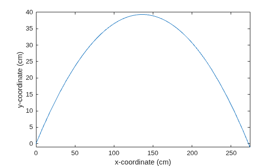
Plot the projectile trajectory using fplot. Set the time range to [0 0.57] seconds. The plot shows the characteristic parabolic trajectory of projectile motion, with the $x$- and $y$-coordinates both in centimeters.

fplot(x,y,[0 0.57])
xlabel(['x-coordinate (',symunit2str(x_units),')'])
ylabel(['y-coordinate (',symunit2str(y_units),')'])

Solve Equation Involving Units

You can solve algebraic equations involving units by using the solve function. This example shows how to solve an equation involving units for the motion of a harmonic oscillator.

Define the symbolic variable for time, and specify the physical parameters of the oscillator with their respective units.

u = symunit;
syms t_wUnit
A = 6*u.cm;
f = 20*u.Hz;
phi = 0.5*u.rad;

Define the displacement of the harmonic oscillator.

y = A*sin(2*pi*f*t_wUnit + phi)

y = 
$$6\hspace{0.17em}\sin \left(40\hspace{0.17em}\pi \hspace{0.17em}{t}_{\mathrm{wUnit}}\hspace{0.17em}\mathrm{Hz}\mathrm{"hertz\; -\; a\; physical\; unit\; of\; frequency."}+\frac{1}{2}\right)\hspace{0.17em}\mathrm{cm}\mathrm{"centimeter\; -\; a\; physical\; unit\; of\; length."}$$

Suppose you want to find the time when the displacement equals 30 millimeters. Define the equation to solve.

eqn = y == 30*u.mm

eqn = 
$$6\hspace{0.17em}\sin \left(40\hspace{0.17em}\pi \hspace{0.17em}{t}_{\mathrm{wUnit}}\hspace{0.17em}\mathrm{Hz}\mathrm{"hertz\; -\; a\; physical\; unit\; of\; frequency."}+\frac{1}{2}\right)\hspace{0.17em}\mathrm{cm}\mathrm{"centimeter\; -\; a\; physical\; unit\; of\; length."}=30\hspace{0.17em}\mathrm{mm}\mathrm{"millimeter\; -\; a\; physical\; unit\; of\; length."}$$

Solve the equation, returning all possible solutions and any associated parameters or conditions.

[sols,param,cond] = solve(eqn,t_wUnit,ReturnConditions=true)

sols = 
$$\left(\begin{array}{c}\frac{\mathrm{asin}\left(5\hspace{0.17em}\frac{\mathrm{mm}\mathrm{"millimeter\; -\; a\; physical\; unit\; of\; length."}}{\mathrm{cm}\mathrm{"centimeter\; -\; a\; physical\; unit\; of\; length."}}\right)+2\hspace{0.17em}\pi \hspace{0.17em}k-\frac{1}{2}}{40\hspace{0.17em}\pi }\hspace{0.17em}\frac{1}{\mathrm{Hz}\mathrm{"hertz\; -\; a\; physical\; unit\; of\; frequency."}}\\ -\frac{\pi +\mathrm{asin}\left(5\hspace{0.17em}\frac{\mathrm{mm}\mathrm{"millimeter\; -\; a\; physical\; unit\; of\; length."}}{\mathrm{cm}\mathrm{"centimeter\; -\; a\; physical\; unit\; of\; length."}}\right)+2\hspace{0.17em}\pi \hspace{0.17em}k+\frac{1}{2}}{40\hspace{0.17em}\pi }\hspace{0.17em}\frac{1}{\mathrm{Hz}\mathrm{"hertz\; -\; a\; physical\; unit\; of\; frequency."}}\end{array}\right)$$

param = $$k$$

cond = 
$$\left(\begin{array}{c}k\in \mathbb{Z}\\ k\in \mathbb{Z}\end{array}\right)$$

Simplify the first solution and convert the result to milliseconds.

t1 = simplify(sols(1))

t1 = 
$$\frac{\pi +12\hspace{0.17em}\pi \hspace{0.17em}k-3}{240\hspace{0.17em}\pi }\hspace{0.17em}\frac{1}{\mathrm{Hz}\mathrm{"hertz\; -\; a\; physical\; unit\; of\; frequency."}}$$

t1 = unitConvert(t1,u.ms)

t1 = 
$$\frac{25\hspace{0.17em}\left(\pi +12\hspace{0.17em}\pi \hspace{0.17em}k-3\right)}{6\hspace{0.17em}\pi }\hspace{0.17em}\mathrm{ms}\mathrm{"millisecond\; -\; a\; physical\; unit\; of\; time."}$$

Use Units in Differential Equations

You can work with differential equations that include units by using the diff, int, and dsolve functions. This example starts from the definition of acceleration and derives the velocity relation $v\left(t\right)=v_0+at$ and the displacement relation $s\left(t\right)=v_{0}t+\frac{1}{2}a{t}^2$.

Define the acceleration, velocity, and time symbolically in SI units.

u = symunit;
syms a v(t)
a_mps2 = a*u.m/u.s^2;
v_mps = v(t)*u.m/u.s;
t_s = t*u.s;

Derive the velocity relation. Define a symbolic equation that relates the acceleration a_mps2 to the velocity v_mps. Because both acceleration and velocity have units, differentiate v_mps with respect to t_s, which also has units.

eqn1 = a_mps2 == diff(v_mps,t_s)

eqn1 = 
$$a\hspace{0.17em}\frac{\mathrm{m}\mathrm{"meter\; -\; a\; physical\; unit\; of\; length."}}{{\mathrm{s}\mathrm{"second\; -\; a\; physical\; unit\; of\; time."}}^2}=\frac{\partial }{\partial t}\mathrm{ }v\left(t\right)\hspace{0.17em}\frac{\mathrm{m}\mathrm{"meter\; -\; a\; physical\; unit\; of\; length."}}{{\mathrm{s}\mathrm{"second\; -\; a\; physical\; unit\; of\; time."}}^2}$$

Solve eqn1 for v(t) with the condition that the initial velocity is $v_0$. The result is the velocity relation $v\left(t\right)=v_0+at$, where $$v(t)$$, $$v_0$$, $$a$$, and $$t$$ are all dimensionless.

syms v_0
cond = v(0) == v_0;
v(t) = dsolve(eqn1,cond)

v(t) = $$v_0+a\hspace{0.17em}t$$

Next, derive the displacement equation. Use the result for v(t) to redefine v_mps. Define a symbolic equation that relates the velocity v_mps to the displacement s_m in SI units.

syms s(t)
s_m = s(t)*u.m;
v_mps = v(t)*u.m/u.s;
eqn2 = v_mps == diff(s_m,t_s)

eqn2 = 
$$\left(v_0+a\hspace{0.17em}t\right)\hspace{0.17em}\frac{\mathrm{m}\mathrm{"meter\; -\; a\; physical\; unit\; of\; length."}}{\mathrm{s}\mathrm{"second\; -\; a\; physical\; unit\; of\; time."}}=\frac{\partial }{\partial t}\mathrm{ }s\left(t\right)\hspace{0.17em}\frac{\mathrm{m}\mathrm{"meter\; -\; a\; physical\; unit\; of\; length."}}{\mathrm{s}\mathrm{"second\; -\; a\; physical\; unit\; of\; time."}}$$

Solve eqn2 for s(t) with the condition that the initial displacement is 0.

cond2 = s(0) == 0;
s(t) = dsolve(eqn2,cond2)

s(t) = 
$$\frac{a\hspace{0.17em}{t}^2}{2}+v_0\hspace{0.17em}t$$

Convert Symbolic Functions with Units to MATLAB Functions

You can generate a MATLAB function from a symbolic expression by first separating the units from the expression with separateUnits and then converting the expression with matlabFunction. This example shows how to convert symbolic functions containing units to MATLAB functions, demonstrating the warning that occurs when units are present and how to handle units.

Define a symbolic function that represents the height of 1-D projectile motion. Specify the projectile's initial vertical speed as 10 kilometers per hour, the gravitational acceleration as 9.81 meters per second squared, and the time variable as an unknown value in seconds. To reflect the physical context, assume the dimensionless time variable t is always positive.

u = symunit;
syms t positive
v0_kph = 10*u.km/u.h;
g_mps2 = 9.81*u.m/u.s^2;
t_s = t*u.s;

Define the height of the projectile as a function of time.

h(t) = v0_kph*t_s - 1/2*g_mps2*t_s^2

h(t) = 
$$10\hspace{0.17em}t\hspace{0.17em}\frac{\mathrm{km}\mathrm{"kilometer\; -\; a\; physical\; unit\; of\; length."}\hspace{0.17em}\mathrm{s}\mathrm{"second\; -\; a\; physical\; unit\; of\; time."}}{\mathrm{h}\mathrm{"hour\; -\; a\; physical\; unit\; of\; time."}}-\frac{981\hspace{0.17em}{t}^2}{200}\hspace{0.17em}\mathrm{m}\mathrm{"meter\; -\; a\; physical\; unit\; of\; length."}$$

Because the formula for the height contains mixed units, convert the length and time dimensions in the formula to centimeters and seconds.

h_cm(t) = unitConvert(h,[u.cm u.s])

h_cm(t) = 
$$\frac{2500\hspace{0.17em}t}{9}\hspace{0.17em}\mathrm{cm}\mathrm{"centimeter\; -\; a\; physical\; unit\; of\; length."}-\frac{981\hspace{0.17em}{t}^2}{2}\hspace{0.17em}\mathrm{cm}\mathrm{"centimeter\; -\; a\; physical\; unit\; of\; length."}$$

Next, convert the symbolic function h_cm to an anonymous MATLAB function using matlabFunction. Because matlabFunction cannot handle symbolic units in the generated code, it replaces the length unit in centimeters with 1 after verifying that the units of the expression are consistent.

hfunc_cm = matlabFunction(h_cm)

Warning: Argument has units. Use 'separateUnits' to remove units before generating code from symbolic expressions.

Warning: Unit 'symunit('cm')' is not supported. Replacing it with '1' after verifying that units of expression are consistent.

hfunc_cm = function_handle with value:
    @(t)t.^2.*1.*(-9.81e+2./2.0)+t.*1.*2.777777777777778e+2

Using this anonymous function, evaluate the height at 0.2 second. Although the result is a numeric value without units, the result implies that the length unit is centimeters.

h_val = hfunc_cm(0.2)

h_val = 
35.9356

To avoid the warning when using matlabFunction, you can use separateUnits to extract the unitless expression. For example, extract the unitless expression after converting the length dimension to meters.

[h_m,h_units] = separateUnits(unitConvert(h_cm,u.m))

h_m(t) = 
$$-\frac{t\hspace{0.17em}\left(8829\hspace{0.17em}t-5000\right)}{1800}$$

h_units(t) = $$\mathrm{m}\mathrm{"meter\; -\; a\; physical\; unit\; of\; length."}$$

Generate a MATLAB function from the unitless expression.

hfunc_m = matlabFunction(h_m)

hfunc_m = function_handle with value:
    @(t)t.*(t.*8.829e+3-5.0e+3).*(-5.555555555555556e-4)

Evaluate the height at 0.2 second. The result implies that the length unit is meters.

h_val = hfunc_m(0.2)

h_val = 
0.3594

Apply Statistical Functions to Vectors with Symbolic Units

You can apply statistical functions, such as mean, median, max, min, std, and var, to vectors with symbolic units by using a helper function. This example shows how to use a helper function to handle unit conversion and separation when applying statistical functions. For the complete code of the applyStatistics helper function, see Helper Function.

Define a vector with different length units.

u = symunit;
l_mixedUnits = [2*u.m + 4*u.in, 3*u.cm, 0.4*u.ft]

l_mixedUnits = 
$$\left(\begin{array}{ccc}4\hspace{0.17em}\mathrm{in}\mathrm{"inch\; -\; a\; physical\; unit\; of\; length."}+2\hspace{0.17em}\mathrm{m}\mathrm{"meter\; -\; a\; physical\; unit\; of\; length."}& 3\hspace{0.17em}\mathrm{cm}\mathrm{"centimeter\; -\; a\; physical\; unit\; of\; length."}& \frac{2}{5}\hspace{0.17em}\mathrm{ft}\mathrm{"foot\; -\; a\; physical\; unit\; of\; length."}\end{array}\right)$$

Find the median and convert the result to inches.

l_median = applyStatistics("median",l_mixedUnits,u.in)

l_median = 
$$\frac{24}{5}\hspace{0.17em}\mathrm{in}\mathrm{"inch\; -\; a\; physical\; unit\; of\; length."}$$

Find the maximum and convert the result to meters.

l_max = applyStatistics("max",l_mixedUnits,u.m)

l_max = 
$$\frac{2627}{1250}\hspace{0.17em}\mathrm{m}\mathrm{"meter\; -\; a\; physical\; unit\; of\; length."}$$

Find the mean and convert the result to centimeters.

l_mean = applyStatistics("mean",l_mixedUnits,u.cm)

l_mean = 
$$\frac{28169}{375}\hspace{0.17em}\mathrm{cm}\mathrm{"centimeter\; -\; a\; physical\; unit\; of\; length."}$$

Find the standard deviation and convert the result to feet.

l_std = applyStatistics("std",l_mixedUnits,u.ft)

l_std = 
$$\frac{\sqrt{3}\hspace{0.17em}\sqrt{642117871}}{11430}\hspace{0.17em}\mathrm{ft}\mathrm{"foot\; -\; a\; physical\; unit\; of\; length."}$$

Helper Function

The applyStatistics helper function handles unit conversion and checks if all elements have compatible units before applying a statistical function.

function value = applyStatistics(funcName,inputVector,outputUnit)
% APPLYSTATISTICS Apply statistical function to vector with symbolic units
%   VALUE = APPLYSTATISTICS(FUNCNAME,INPUTVECTOR,OUTPUTUNIT) applies the
%   statistical function specified by FUNCNAME to INPUTVECTOR, which
%   contains elements with symbolic units. The result is returned in the
%   units specified by OUTPUTUNIT.
%
%   Inputs:
%       funcName     - String or character vector specifying the statistical
%                      function to apply (such as "mean", "median", "max",
%                      "min", "std", "var")
%       inputVector  - Vector containing symbolic expressions with units
%       outputUnit   - Symbolic unit for the output value (optional). If not
%                      specified, uses the unit of the first element
%
%   Output:
%       value        - Result of applying the statistical function to the
%                      input vector, expressed in the specified output unit
%
%   Example:
%       u = symunit;
%       data = [2*u.m, 150*u.cm, 0.5*u.m];
%       avgValue = applyStatistics("mean",data,u.cm)
%
%   See also SYMUNIT, UNITCONVERT, SEPARATEUNITS, CHECKUNITS

% Check if input is empty
if isempty(inputVector)
    error("Input vector cannot be empty");
end
    
% Separate units from the input data to get the units
[~,units] = separateUnits(inputVector);
    
% If no output unit specified, use the unit of first element as a reference
if nargin < 3
    outputUnit = units(1);
end
    
% Check that all elements have compatible units
expr = sum(units) + outputUnit;
if ~checkUnits(expr,"Compatible")
    error("All units in the input and target unit must be compatible.");
end

% Convert all values to the output unit for comparison
convertedElements = unitConvert(inputVector,outputUnit);
[convertedValues,~] = separateUnits(convertedElements);

% Apply function to values
value = feval(funcName,convertedValues);

% Return value with specified unit
value = value*outputUnit;
end