opticalFlowRAFT

Estimate optical flow using RAFT deep learning algorithm

Since R2024b

Description

Use the opticalFlowRAFT object to estimate the motion direction and velocity between previous and current video frames using the recurrent all-pairs field transforms (RAFT) algorithm. This algorithm uses a deep learning network trained on the Kubric [3] dataset. The RAFT optical flow estimation algorithm outperforms approaches like Farneback by delivering greater accuracy, particularly in areas with minimal texture, motion blur, and under difficult camera movements. It provides dense (per-pixel) and highly accurate estimations, but requires more time and memory. For quicker but less precise dense optical flow estimation, opt for opticalFlowFarneback, a traditional vision algorithm that does not rely on deep learning.

Note

This functionality requires Deep Learning Toolbox™ and the Computer Vision Toolbox™ Model for RAFT Optical Flow Estimation. You can install the Computer Vision Toolbox Model for RAFT Optical Flow Estimation from Add-On Explorer. For more information about installing add-ons, see Get and Manage Add-Ons.

Creation

Syntax

flowModel = opticalFlowRAFT

Description

flowModel = opticalFlowRAFT returns an optical flow object that estimates the motion direction and velocity between the previous and current video frames.

Object Functions

estimateFlow	Estimate optical flow between two frames
reset	Reset the internal state of the optical flow estimation object

Examples

Estimate Optical Flow in Consecutive Image Frames

Create a RAFT optical flow object.

flowModel = opticalFlowRAFT;

Create an object to read the input video file.

vidReader = VideoReader("visiontraffic.avi",CurrentTime=11);

Create a custom figure window to visualize the optical flow vectors.

h = figure;
movegui(h);
hViewPanel = uipanel(h, Position=[0 0 1 1], Title="Plot of Optical Flow Vectors");
hPlot = axes(hViewPanel);

Read consecutive image frames to estimate optical flow. Display the current frame and overlay optical flow vectors using a quiver plot. The estimateFlow function calculates the optical flow between two consecutive frames.

Note that the function internally stores the previous frame and utilizes it implicitly for optical flow estimation. Consequently, when the function is called for the first time on a sequence of frames, it will return a zero flow. This is because, in the absence of a genuine previous frame, the initial frame is treated as both the current and previous frame, leading to no detectable motion between the two. This is consistent with the argument structure and behavior of established optical flow estimation methods, such as opticalFlowFarneback.

while hasFrame(vidReader)
    frame = readFrame(vidReader);
    flow = estimateFlow(flowModel,frame);

    imshow(frame)
    hold on
    plot(flow,DecimationFactor=[10 10],ScaleFactor=0.45,Parent=hPlot,color="g");
    hold off
    pause(10^-3)
end

Reset the opticalFlowRAFT object after the video processing has completed. This clears the internal state of the object, including the saved previous frame.

reset(flowModel);

Memory-Efficient RAFT Optical Flow for Large Images Using Rescaling

RAFT provides accurate optical flow estimation, but it can be memory-intensive when applied to large images or run on GPUs with limited memory. In such cases, processing high-resolution frames directly may lead to out-of-memory (OOM) errors. A practical solution is to downscale the input images before passing them to the RAFT model, compute optical flow at the reduced resolution, and then rescale the resulting flow field back to the original size of the imagery. This example demonstrates how to apply this memory-efficient strategy, allowing you to use RAFT on larger images or resource-constrained hardware while preserving meaningful flow estimates.

Load Image Pair

Load two images and visualize their pixel-wise differences due to camera motion using a red-cyan composite image.

I1 = imread("yellowstone_left.png");
I2 = imread("yellowstone_right.png");

figure
imshow(stereoAnaglyph(I1, I2))
title("Composite Image (Red - Left Image, Cyan - Right Image)")

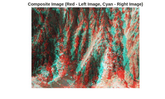
Display the spatial dimensions of the images.

disp(size(I1, [1 2]))

   480   640

Create opticalFlowRAFT Object

Create an opticalFlowRAFT object for computing optical flow between two images.

raft = opticalFlowRAFT;

Estimate Optical Flow on Full Resolution Images

Estimate optical flow on the images at original resolution. This gives the most accurate result but may cause into slow runtime and high memory consumption.

estimateFlow(raft, I1);
flowFull = estimateFlow(raft, I2);

Estimate Optical Flow on Downsampled Images

Create Downscaled Images

Scale the image dimensions by a factor of 0.5 for illustrative purpose. A small resolution image can result in faster optical flow computation and less memory consumption.

I1Small = imresize(I1, 0.5);
I2Small = imresize(I2, 0.5);

Display the resized image dimensions.

disp(size(I1Small, [1 2]))

   240   320

Estimate Flow on Downscaled Images

Compute optical flow on downscaled images. Use the same opticalFlowRAFT model instantiated earlier after resetting it.

reset(raft);
estimateFlow(raft, I1Small);
flowLowRes = estimateFlow(raft, I2Small);

Scale Estimated Flow to Original Resolution

Upsample and scale the lower resolution optical flow back to the original image resolution.

origDims = size(I1, [1 2]);
scaleX = origDims(2) / size(flowLowRes.Magnitude, 2);
scaleY = origDims(1) / size(flowLowRes.Magnitude, 1);

flowX = imresize(flowLowRes.Vx, origDims, "bilinear") * scaleX;
flowY = imresize(flowLowRes.Vy, origDims, "bilinear") * scaleY;

flowUpscaled = opticalFlow(flowX, flowY);

Compare Optical Flow at Original and Downscaled Resolutions

Visually compare optical flow computed directly on the original high-resolution images with optical flow computed on downscaled images and then rescaled back to the original size. This comparison illustrates how the downscale-upscale workflow approximates the original flow while reducing memory usage.

figure
subplot(1,2,1)
imshow(I1)
hold on
plot(flowFull, DecimationFactor=[40 40], ScaleFactor=0.75, Color="g");
hold off
title("Optical Flow at Full Resolution")

subplot(1,2,2)
imshow(I1)
hold on
plot(flowUpscaled, DecimationFactor=[40 40], ScaleFactor=0.75, Color="g");
hold off
title("Optical Flow at Half Resolution")

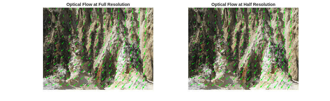
The bilinear interpolation in the image resizing operations can introduce numerical inaccuracies and overly-smoothed results in the upscaled optical flow. This reduced accuracy is a trade-off against the lower memory consumption when optical flow computation is performed on lower resolution imagery.

References

[1] Teed, Zachary, and Jia Deng. RAFT: Recurrent All-Pairs Field Transforms for Optical Flow. Proceedings of the 16th European Conference on Computer Vision. 2020.

[2] Shah, Neelay, Prajnan Goswami, and Huaizu Jiang. EzFlow: A modular PyTorch library for optical flow estimation using neural networks. 2021. Web. https://github.com/neu-vi/ezflow.

[3] Greff, Klaus, Francois Belletti, Lucas Beyer, Carl Doersch, Yilun Du, Daniel Duckworth, David J. Fleet et al. Kubric: A scalable dataset generator. In Proceedings of the IEEE/CVF conference on computer vision and pattern recognition, pp. 3749-3761. 2022.

Version History

Introduced in R2024b