Localize Screen Manufacturing Defects Using Student-Teacher Anomaly Detector
R2026bThis example shows how to train a Student-Teacher anomaly detection network on normal phone screen images, select an anomaly threshold by using a calibration set, and evaluate the detector on test images containing manufacturing defects.
The Student-Teacher model is a one-class anomaly detector that you train by using only normal (non-anomalous) images. A pretrained teacher network extracts features that characterize normal data, and a student network learns to replicate those features. At inference time, you identify anomalies by comparing the per-pixel discrepancy between the student and teacher outputs. Image pixels where the student fails to predict the teacher features correspond to defects. The high accuracy, low latency, and high throughput of the Student-Teacher model enables you to localize defects in large-scale applications that require real-time response.
Download Pretrained Student-Teacher Detector
By default, this example downloads a pretrained Student-Teacher anomaly detector by using the downloadTrainedNetwork helper function. This function is attached to this example as a supporting file. You can use the pretrained network to run the entire example without waiting for training to complete.
trainedScreenDefectDetectorNetURL = "https://ssd.mathworks.com/supportfiles/" + ...
     "visualinspection/data/trainedScreenDefectDetectorModel.zip";
downloadTrainedNetwork(trainedScreenDefectDetectorNetURL,pwd)
Network extracted successfully.
load("trainedScreenDefectDetectorModel.mat")Download MulSen-AD and MulSenAug-AD Data Sets
This example uses the screen RGB subset of the MulSen-AD [1] data set, a high-resolution multi-sensor anomaly detection data set for industrial applications. The MulSenAug-AD data set augments MulSen-AD with synthetic images to increase the training set size. Anomalous test images contain screen defects such as scratches, cracks, and broken parts.
The data subsets contain train and test folders with normal training images and normal and anomalous test images, respectively. Specify dataDir as the location of the data set. Download the data set by using the downloadMulSenADScreenData and downloadMulSenAugADScreenData helper functions. These functions are attached to this example as supporting files.
dataDir = fullfile(tempdir,"MulSenAD_DataSet");
MulsenADURL = "https://ssd.mathworks.com/supportfiles/" + ...
    "visualinspection/data/MulSenAD.zip";
downloadMulSenADScreenData(MulsenADURL,dataDir + "/MulSenAD")
MulsenAugADURL = "https://ssd.mathworks.com/supportfiles/" + ...
    "visualinspection/data/MulSenAugAD.zip";
downloadMulSenAugADScreenData(MulsenAugADURL,dataDir + "/MulSenAugAD")
Localize Defects in Image
Read a sample anomalous image with a "broken" label from the data set. Apply the same preprocessing that was applied to the pretrained detector training data: rescale pixel values to the range [0,1] and convert them to the single data type prior to training.
sampleImage = imread(fullfile(dataDir,"MulSenAD", ...
    "screen","RGB","test","broken","1.png"));
sampleImage = im2single(sampleImage);
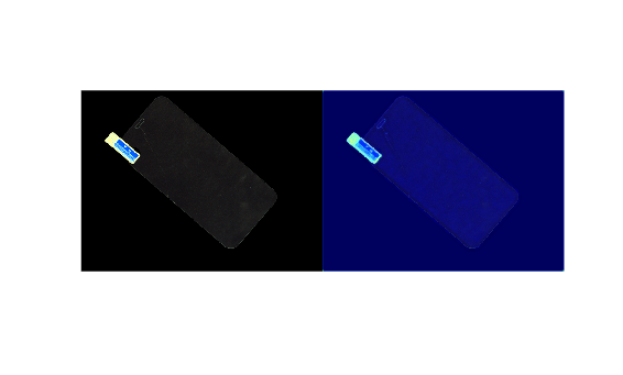
Visualize defect localization by overlaying the predicted per-pixel anomaly score map on the sample image. Use the anomalyMap function to generate the anomaly score heatmap. Adjust the contrast of the brightness channel to improve the visibility of the screen image from the background. Display the image with the heatmap overlaid by using the anomalyMapOverlay function.
anomalyHeatMap = anomalyMap(detector,sampleImage);
sampleImage = adjustContrast(sampleImage);
heatMapImage = anomalyMapOverlay(sampleImage,anomalyHeatMap);
montage({sampleImage,heatMapImage})
title("Heatmap of Anomalous Image")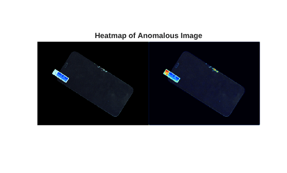
Prepare Data for Training
Create ImageDatastore objects from the train and test folders of the downloaded MulSenAugAD screen data set.
rng("default")
trainDataDir = fullfile(dataDir,"MulSenAD","screen","RGB","train");
trainAugDataDir = fullfile(dataDir,"MulSenAugAD","screen","RGB","train");
dsTrain = imageDatastore([trainDataDir trainAugDataDir],IncludeSubfolders=true,LabelSource="foldernames",FileExtensions=".png");
testDataDir = fullfile(dataDir,"MulSenAD","screen","RGB","test");
testAugDataDir = fullfile(dataDir,"MulSenAugAD","screen","RGB","test");
dsData = imageDatastore([testDataDir testAugDataDir],IncludeSubfolders=true,LabelSource="foldernames",FileExtensions=".png");
Define the normal class label. The data set stores normal images in a folder named "good".
normalClasses = categorical("good");
uniqueClasses = unique(dsData.Labels);
anomalyClasses = uniqueClasses(~ismember(uniqueClasses,normalClasses));
Split the test data into calibration and test sets by using the splitAnomalyData function.
[~,dsCal,dsTest] = splitAnomalyData(dsData,anomalyClasses,DataAllocationRatio=[0 0.2 0.8]);
Splitting anomaly dataset
-------------------------
* Finalizing... Done.
* Number of files and proportions per class in all the datasets:

                      Input                 Train              Validation                Test
               ___________________    _________________    ___________________    ___________________

               NumFiles     Ratio     NumFiles    Ratio    NumFiles     Ratio     NumFiles     Ratio
               ________    _______    ________    _____    ________    _______    ________    _______

    broken        32       0.23022       0          0         6        0.22222       26       0.23214
    crack         20       0.14388       0          0         4        0.14815       16       0.14286
    good          33       0.23741       0          0         7        0.25926       26       0.23214
    label         20       0.14388       0          0         4        0.14815       16       0.14286
    scratch       34        0.2446       0          0         6        0.22222       28          0.25
Display a normal screen image and an anomalous screen image from the test data set.
anomalyImage = find(dsTest.Labels==anomalyClasses(1),1);
anomalyImage = read(subset(dsTest,anomalyImage));
normalImage = find(dsTest.Labels==normalClasses(1),1);
normalImage = read(subset(dsTest,normalImage));
normalImage = adjustContrast(normalImage);
anomalyImage = adjustContrast(anomalyImage);
montage({normalImage,anomalyImage})
title("Screen images without (left) and with (right) defects")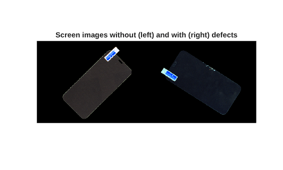
Partition Data into Calibration and Test Sets
Use a calibration set to determine the threshold for the classifier. Separate calibration and test sets prevent information from the test set from leaking into the classifier design. The classifier labels images with anomaly scores above the threshold as anomalous.
To establish a suitable threshold for the classifier, allocate 20% of the test data as the calibration set dsCal and 80% as the test set dsTest.
Apply one-hot encoding labels to the training, calibration, and test datastores by using the addLabelData supporting function.
dsTrain = transform(dsTrain,@(x,y)addLabelData(x,y,normalClasses),IncludeInfo=true);
dsCal = transform(dsCal,@(x,y)addLabelData(x,y,normalClasses),IncludeInfo=true);
dsTest = transform(dsTest,@(x,y)addLabelData(x,y,normalClasses),IncludeInfo=true);
imgData = preview(dsTrain);
fprintf("The size of the train images: %s\n",strjoin(string(size(imgData{1}))," x "));
The size of the train images: 960 x 1280 x 3
fprintf("Number of train images: %d\n",dsTrain.numpartitions);Number of train images: 386
Define Student-Teacher Anomaly Detector Network Architecture
Create a Student-Teacher anomaly detector network by using the studentTeacherAnomalyDetector object.
studentTeacher = studentTeacherAnomalyDetector(Network="small");Train Detector
To train the detector, set the doTraining variable to true. Train the detector by using the trainStudentTeacherAnomalyDetector function with the untrained studentTeacher network and the training data as inputs.
Train on one or more GPUs, if they are available. Using a GPU requires a Parallel Computing Toolbox™ license and a CUDA®-enabled NVIDIA® GPU. For more information, see GPU Computing Requirements (Parallel Computing Toolbox).
doTraining =false; if doTraining maximumEpochs=20; options = trainingOptions("adam", ... ExecutionEnvironment="auto", ... InitialLearnRate=1e-4,... L2Regularization=1e-5',... LearnRateSchedule="piecewise", ... LearnRateDropPeriod=floor(0.9*maximumEpochs), ... LearnRateDropFactor=0.1, ... MaxEpochs=maximumEpochs, ... VerboseFrequency=2, ... MiniBatchSize=2, ... Shuffle="every-epoch", ... ValidationData=dsCal, ... OutputNetwork="best-validation", ... Metrics=aucMetric(Name="auc"), ... ObjectiveMetricName="auc", ... ResetInputNormalization=true,... Plots="training-progress", ... PreprocessingEnvironment="background"); detector = trainStudentTeacherAnomalyDetector(dsTrain,studentTeacher,options,AnomalyMapNormalizationDataRatio=0.2); end
Set Anomaly Threshold
An important stage of semi-supervised anomaly detection is choosing an anomaly score threshold. The detector classifies images as anomalous when their scores exceed this threshold. This example uses a calibration data set, defined in the Partition Data into Calibration and Test Sets section, that contains both normal and anomalous images to select the threshold.
Obtain the anomaly score for each image in the calibration set by using the predict object function. Extract the ground truth labels.
scores = predict(detector,dsCal,MiniBatchSize=1);
labels = dsCal.UnderlyingDatastores{1}.Labels ~= normalClasses;
Plot a histogram of the anomaly scores for the normal and anomalous classes. The distributions are well separated by the model-predicted anomaly score.
numBins = 20;
[~,edges] = histcounts(scores,numBins);
figure
hold on
hNormal = histogram(scores(labels==0),edges);
hAnomaly = histogram(scores(labels==1),edges);
hold off
legend([hNormal,hAnomaly],"Normal","Anomaly")
xlabel("Anomaly Score")
ylabel("Counts")
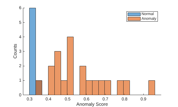
Calculate the optimal anomaly threshold by using the anomalyThreshold function. Specify the first two input arguments as the ground truth labels, labels, and predicted anomaly scores, scores, for the calibration data set. Specify the third input argument as true because true positive anomaly images have a labels value of true. The anomalyThreshold function returns the optimal threshold value as a scalar and the receiver operating characteristic (ROC) curve for the detector as an rocmetrics (Deep Learning Toolbox) object.
[thresh,roc] = anomalyThreshold(labels,scores,true,"MaxF1Score");Set the Threshold property of the anomaly detector to the optimal value.
detector.Threshold = thresh;
Plot the ROC curve by using the plot (Deep Learning Toolbox) object function of rocmetrics. The ROC curve illustrates classifier performance across a range of threshold values. Each point represents the false positive rate (x-coordinate) and true positive rate (y-coordinate) for a given threshold. The area under the ROC curve (AUC) indicates classifier performance, where a value of 1.0 corresponds to a perfect classifier.
plot(roc)
title("ROC AUC: "+ roc.AUC)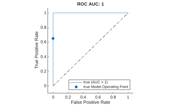
After threshold selection using the calibration data, obtain the anomaly score and ground truth label for each image in the test set to determine how well the selected threshold generalizes to the test data.
scores = predict(detector,dsTest,MiniBatchSize=1);
labels = dsTest.UnderlyingDatastores{1}.Labels ~= normalClasses;
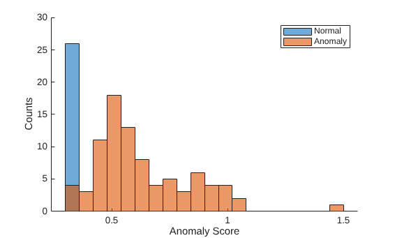
Plot a histogram of the anomaly scores for the normal and anomalous classes in the test set. Verify that the selected threshold separates the score distributions for the test data.
numBins = 20;
[~,edges] = histcounts(scores,numBins);
figure
hold on
hNormal = histogram(scores(labels==0),edges);
hAnomaly = histogram(scores(labels==1),edges);
hold off
legend([hNormal,hAnomaly],"Normal","Anomaly")
xlabel("Anomaly Score")
ylabel("Counts")
Evaluate Classification Model
Classify each image in the test set as either normal or anomalous by using the classify object function.
testSetPredictedLabels = classify(detector,dsTest,MiniBatchSize=1);
testSetPredictedLabels = testSetPredictedLabels';
Get the ground truth labels of each test image.
testSetGTLabels = dsTest.UnderlyingDatastores{1}.Labels;Evaluate the anomaly detector by calculating performance metrics by using the evaluateAnomalyDetection function. The function calculates several metrics that evaluate the accuracy, precision, sensitivity, and specificity of the detector for the test data set.
metrics = evaluateAnomalyDetection(testSetPredictedLabels,testSetGTLabels,anomalyClasses);
Evaluating anomaly detection results
------------------------------------
* Finalizing... Done.
* Data set metrics:

    GlobalAccuracy    MeanAccuracy    Precision    Recall     Specificity    F1Score    FalsePositiveRate    FalseNegativeRate
    ______________    ____________    _________    _______    ___________    _______    _________________    _________________

       0.94643          0.96512           1        0.93023         1         0.96386            0                0.069767
Extract the confusion matrix from the ConfusionMatrix property of metrics and display a confusion plot.
M = metrics.ConfusionMatrix{:,:};
confusionchart(M,["Normal","Anomaly"])
acc = sum(diag(M)) / sum(M,"all");
title("Accuracy: "+acc)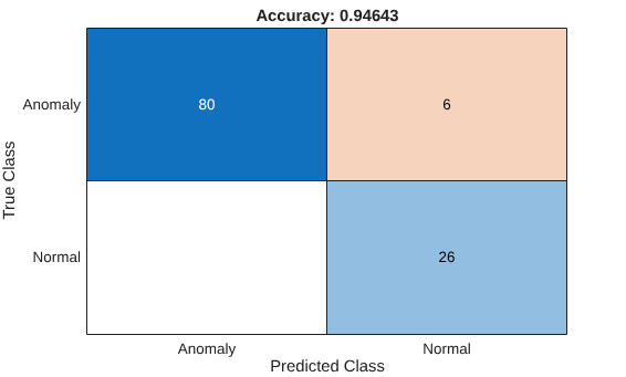
Save Trained Model
Save the trained detector to a MAT file with a timestamp for future use.
if doTraining
    modelDateTime = string(datetime("now",Format="yyyy-MM-dd-HH-mm-ss"));
    save(string(pwd)+filesep+"trainedMulSenAugADScreenDefectDetectorStudentTeacherModel"+modelDateTime+".mat", ...
        "detector");
end
Explain Classification Decisions
The predicted anomaly heatmap explains why the detector classifies an image as normal or anomalous. Examine patterns in false negatives and false positives to identify strategies for improving detector performance, such as balancing the training data or adjusting the threshold.
Calculate Anomaly Heat Map Display Range
Calculate a display range that reflects the range of anomaly scores observed across the entire calibration set, including normal and anomalous images. By using the same display range across images, you can compare images more easily than if you scale each image to its own minimum and maximum. Apply the display range for all heatmaps in this example.
minMapVal = inf;
maxMapVal = -inf;
reset(dsCal)
while hasdata(dsCal)
    img = read(dsCal);
    img = img{1};
    map = anomalyMap(detector,img);
    minMapVal = min(min(map,[],"all"),minMapVal);
    maxMapVal = max(max(map,[],"all"),maxMapVal);
end
displayRange = [minMapVal 0.7*maxMapVal];
View Heatmap of Anomalous Image
Select an image of a correctly classified anomaly. Display the image with the heatmap overlaid by using the anomalyMapOverlay function.
testSetGTLabelsLogical = testSetGTLabels ~= normalClasses;
idxTruePositive = find(testSetGTLabelsLogical & testSetPredictedLabels);
dsExample = subset(dsTest,idxTruePositive);
data = read(dsExample);
img = data{1};
map = anomalyMap(detector,img);
img = adjustContrast(img);
overlayImg = anomalyMapOverlay(img,map,MapRange=displayRange,Blend="equal");
montage({img,overlayImg});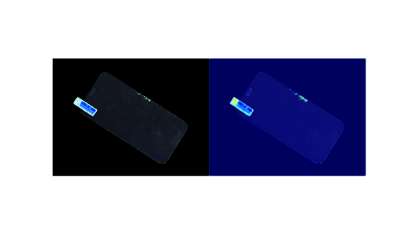
View Heatmap of Normal Image
Select and display a correctly classified normal image with the heatmap overlaid.
idxTrueNegative = find(~(testSetGTLabelsLogical | testSetPredictedLabels));
dsExample = subset(dsTest,idxTrueNegative);
data = read(dsExample);
img = data{1};
map = anomalyMap(detector,img);
img = adjustContrast(img);
overlayImg = anomalyMapOverlay(img,map,MapRange=displayRange,Blend="equal");
montage({img,overlayImg});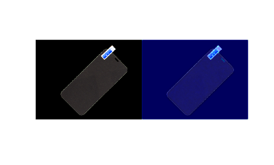
View Heatmap of False Positive Image
False positives are normal images that the detector incorrectly classifies as anomalous. For this pretrained model and test set, no false positives occur. If your data produces false positives, the heatmap reveals which image regions trigger the misclassification. Common strategies to reduce false positives include adjusting image contrast during preprocessing, increasing the number of training images, or choosing a different threshold at the calibration step.
idxFalsePositive = find(~(testSetGTLabelsLogical) & testSetPredictedLabels);
if ~isempty(idxFalsePositive)
    dsExample = subset(dsTest,idxFalsePositive);
    data = read(dsExample);
    img = data{1};
    map = anomalyMap(detector,img);
    img = adjustContrast(img);
    overlayImg = anomalyMapOverlay(img,map,MapRange=displayRange,Blend="equal");
    montage({img,overlayImg});
end
View Heatmap of False Negative Image
False negatives are anomalous images that the detector incorrectly classifies as normal. Use the heatmap to gain insight into the misclassifications.
Find and display a false negative image with the heatmap overlaid. To decrease false negative results, consider adjusting the anomaly threshold or CompressionRatio of the detector.
idxFalseNegative = find(testSetGTLabelsLogical & (~testSetPredictedLabels));
if ~isempty(idxFalseNegative)
    dsExample = subset(dsTest,idxFalseNegative);
    data = read(dsExample);
    img = data{1};
    map = anomalyMap(detector,img);
    img = adjustContrast(img);
    overlayImg = anomalyMapOverlay(img,map,MapRange=displayRange,Blend="equal");
    montage({img,overlayImg});
end
Supporting Functions
addLabelData
Add one-hot encoding labels to the datastores for training and evaluation.
function [data,info] = addLabelData(data,info,normalClass)
classNames = [info.Label];
onehotencoding = classNames ~= normalClass;
data = im2single(data);
data = {data,onehotencoding};
end
adjustContrast
Adjust the contrast of the brightness channel
function imgContrastAdjusted = adjustContrast(img)
% adjustContrast Adjust the contrast of the brightness channel to improve
% the visibility of the screen image from the background.

% 1. Move image to HSV space
hsvImage = rgb2hsv(img);

% 2. Isolate the 'Value' (brightness) channel
V = hsvImage(:,:,3);

% 3. Adjust the Value channel
adjustedV = imadjust(V,[0 0.3],[]);

% 4. Replace the original Value channel with the adjusted one
hsvImage(:,:,3) = adjustedV;

% 5. Convert back to RGB
imgContrastAdjusted = hsv2rgb(hsvImage);

end
References
[1] Li, Wenqiao, Bozhong Zheng, Xiaohao Xu, Jinye Gan, Fading Lu, Xiang Li, Na Ni et al. "Multi-sensor object anomaly detection: Unifying appearance, geometry, and internal properties." In Proceedings of the computer vision and pattern recognition conference, pp. 9984-9993. 2025.
See Also
studentTeacherAnomalyDetector | trainStudentTeacherAnomalyDetector | anomalyMap | anomalyThreshold | evaluateAnomalyDetection

