removeHarmonics

Remove harmonic interferences using wavelet packet transform

Since R2025a

Syntax

y = removeHarmonics(x,Fh,Fs)

y = removeHarmonics(xt,Fh)

y = removeHarmonics(___,Name=Value)

[y,wpt,info] = removeHarmonics(___)

removeHarmonics(___)

Description

y = removeHarmonics(x,Fh,Fs) removes harmonic interferences with base frequency Fh from x sampled at rate Fs and returns the result. removeHarmonics requires a Signal Processing Toolbox™ license.

removeHarmonics obtains the discrete wavelet packet transform (DWPT) of x down to level ceil(log2(Fs/Fh)) using the orthogonal "sym8" wavelet. For more information, see Wavelet Packet Transform and Baseline Shifting.

y = removeHarmonics(xt,Fh) removes harmonic interferences with base frequency Fh from the data in timetable xt and returns the result. The removeHarmonics function calculates the sample rate from the row times of xt.

For timetable input, if you provide a sample rate, removeHarmonics ignores it.

y = removeHarmonics(___,Name=Value) specifies options using one or more name-value arguments, in addition to the input arguments in previous syntaxes. For example, to specify the orthogonal "sym4" wavelet, the Daubechies least-symmetric wavelet with four vanishing moments, set Wavelet to "sym4".

[y,wpt,info] = removeHarmonics(___) returns the DWPT decomposition after baseline removal in wpt and the corresponding baseline estimation metadata in info.

removeHarmonics(___) plots the power spectra of the input and output signals in decibels in the current figure.

Examples

Remove Harmonic Interferences

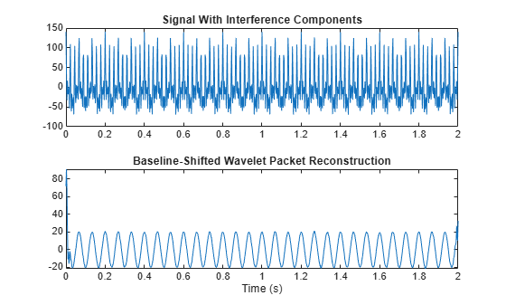
Sample a 15 Hz sinusoidal signal at a rate of 400 Hz for two seconds. The amplitude of the sinusoid is 20. Add noise and harmonic interference components to the signal. The frequency of each interference component is an integer multiple of 45 Hz.

freq = 15;
Fs = 400;
Fh = 45;
t = 0:1/Fs:2;
x = 20*cos(2*pi*freq*t);
harmint = 40*cos(2*pi*Fh*t) + ...
    40*cos(2*pi*2*Fh*t) + ...
    40*cos(2*pi*3*Fh*t);
x = x+harmint+0.5*randn(size(t));

Use removeHarmonics to remove the interferences. The output is a baseline-shifted wavelet packet reconstruction.

y = removeHarmonics(x,Fh,Fs);

Plot the input signal and the reconstruction.

tiledlayout(2,1)
nexttile
plot(t,x)
title("Signal With Interference Components")
nexttile
plot(t,y)
title("Baseline-Shifted Wavelet Packet Reconstruction")
xlabel("Time (s)")

Compare DWPT Decompositions Before and After Harmonic Removal

Create a signal consisting of two sinusoids of frequencies 25 Hz and 140 Hz. Add noise and harmonic interference components to the signal. The base harmonic frequency is 40 Hz. Add first-, second-, third- and fourth-order harmonics. Sample the signal at a rate of 400 Hz for two seconds.

frq1 = 25;
frq2 = 140;
Fh = 40;
Fs = 400;

t = 0:1/Fs:2;
x = sin(2*pi*frq1*t+pi/3)+sin(2*pi*frq2*t);

harmint = 2*sin(2*pi*Fh*t+2*pi/5) + ...
    0.5*sin(2*pi*2*Fh*t) + ...
    sin(2*pi*Fh*3*t+pi/3) + ...
    3*sin(2*pi*Fh*4*t+pi/7);

x = x+harmint+0.1*randn(size(t));

Remove the harmonic interference components from the signal. Use the orthogonal "fk14" wavelet. Obtain the baseline-shifted wavelet packet reconstruction and the DWPT decomposition after baseline removal.

wv = "fk14";
[y,wptRH] = removeHarmonics(x,Fh,Fs,Wavelet=wv);

The removeHarmonics function obtains the DWPT of the signal down to level ceil(log2(Fs/Fh)). Obtain the DWPT coefficients for the original signal down to the same level with the same orthogonal wavelet. Also obtain the center frequencies of the approximate passbands. Because dwpt returns the center frequencies in cycles per second, multiply them by the sample rate to obtain the center frequencies in hertz.

L = ceil(log2(Fs/Fh));
[wptOrig,~,~,cf] = dwpt(x,wv,Level=L);
cf = Fs*cf;

In a DWPT decomposition, all terminal nodes have the same size. Inspect the size of a terminal node in the DWPT decomposition of the original signal and after baseline removal. The terminal node in the second decomposition is larger because the input signal was resampled at a rate of $$\text{Fh}\times 2^L$$ Hz. For more information, see Wavelet Packet Transform and Baseline Shifting.

size(wptOrig{1})

ans = 1×2

     1    62

size(wptRH{1})

ans = 1×2

     1    81

For each decomposition, concatenate the nodes and plot them. The nodes are in sequency order. Label the x-axis with the corresponding center frequency of the approximate passbands. Use the helper function helperPlotDWPTNodes.

helperPlotDWPTNodes(wptOrig,"Original Signal Decomposition",Fs,cf)

helperPlotDWPTNodes(wptRH,"Decomposition After Baseline Removal",Fh*2^L)

Obtain the DWPT decomposition of the reconstructed signal and plot the terminal node coefficients. Compare this decomposition with the DWPT of the original signal. Each node corresponds to an approximate passband. If the corresponding center frequency is close to a harmonic frequency, the coefficients in the associated node are smaller in the DWPT of the reconstructed signal.

wptRec = dwpt(y,wv,Level=L);
helperPlotDWPTNodes(wptRec,"DWPT of Reconstruction",Fs,cf)

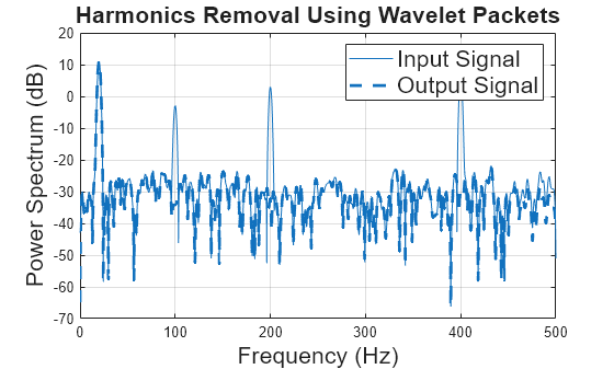
Use removeHarmonics to plot the power spectra of the input signal and output reconstruction. Confirm that the harmonics have been removed.

removeHarmonics(x,Fh,Fs,Wavelet=wv)

Visualize Power Spectra After Interference Removal

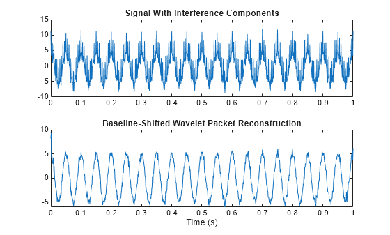
Sample a 30 Hz sinusoid at a rate of 1000 Hz for one second. Add noise and harmonic interference components to the signal. The base harmonic frequency is 100 Hz. Add first-, second-, and fourth-order harmonics.

freq = 20;
Fs = 1000;
t = 0:1/Fs:1;
x = 5*cos(2*pi*freq*t);

Fh = 100;
harmint = cos(2*pi*1*Fh*t) + ...
    2*cos(2*pi*2*Fh*t) + ...
    3*cos(2*pi*4*Fh*t);
 
x = x+harmint+0.5*randn(size(t));

Remove the interference components from the signal. Obtain the baseline-shifted wavelet packet reconstruction.

y = removeHarmonics(x,Fh,Fs);

Plot the input signal and the reconstruction.

tiledlayout(2,1)
nexttile
plot(t,x)
title("Signal With Interference Components")
nexttile
plot(t,y)
title("Baseline-Shifted Wavelet Packet Reconstruction")
xlabel("Time (s)")

Use removeHarmonics to plot the power spectra of the input signal and output reconstruction. removeHarmonics uses pspectrum (Signal Processing Toolbox) to compute the power spectrum of each signal. pspectrum uses a Kaiser window to compute the spectrum over the entire Nyquist range. The frequency resolution bandwidth depends on the size of the input data. For more information, see Spectrum Computation (Signal Processing Toolbox).

figure
removeHarmonics(x,Fh,Fs)

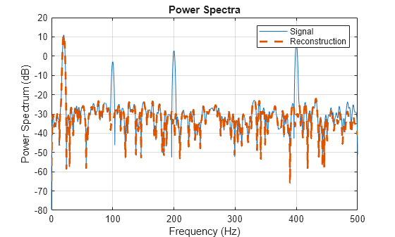
You can recreate the plot using the removeHarmonics output. Use pspectrum to compute the power spectrum of the input signal and reconstruction. Also obtain the spectrum frequencies.

[Pxx,f] = pspectrum(x,Fs);
Pxxy = pspectrum(y,Fs);

Convert the power spectra to dB.

Pxx_db = 10*log10(Pxx);
Pxxy_db = 10*log10(Pxxy);

Plot the power spectra.

plot(f,Pxx_db,LineWidth=0.5)
hold on
plot(f,Pxxy_db,LineWidth=2,LineStyle="--")
hold off
grid on
title("Power Spectra")
legend("Signal","Reconstruction")
xlabel("Frequency (Hz)")
ylabel("Power Spectrum (dB)")

Input Arguments

x — Input signal

vector | matrix

Input signal, specified as a vector or matrix.

If x is a vector, removeHarmonics treats x as a single channel. If x is a matrix, each column represents a channel, and removeHarmonics operates on the columns of x. Each channel of x must have a length greater than or equal to two periods of Fh in samples.

Data Types: single | double

Fh — Base harmonic frequency

positive scalar

Base harmonic frequency in hertz, specified as a positive scalar. The base harmonic frequency must be less than the sample rate, Fs. The removeHarmonics function removes interferences from all integer multiples of Fh no larger than Fs/2.

Data Types: single | double

Fs — Sample rate

positive scalar

Sample rate in hertz, specified as a positive scalar. The sample rate must be greater than the base harmonic frequency, Fh.

Data Types: single | double

xt — Input timetable

timetable

Input timetable. xt can have either a single variable containing a vector or matrix, or multiple variables each containing a vector. removeHarmonics operates on the columns of xt. The timetable must contain increasing, finite, and equally spaced row times of type duration in seconds. The number of rows must be greater than or equal to two periods of Fh in samples.

Data Types: single | double

Name-Value Arguments

Specify optional pairs of arguments as Name1=Value1,...,NameN=ValueN, where Name is the argument name and Value is the corresponding value. Name-value arguments must appear after other arguments, but the order of the pairs does not matter.

Example: y = removeHarmonics(x,Fh,Fs,Boundary="zeropad",Wavelet="fk14")

Wavelet — Orthogonal wavelet

"sym8" (default) | character vector | string scalar

Orthogonal wavelet to use to obtain the DWPT, specified as a character vector or string scalar. Orthogonal wavelets are designated as type 1 wavelets in the wavelet manager, wavemngr.

Valid built-in orthogonal wavelet families are: Best-localized Daubechies ("bl"), Beylkin ("beyl"), Coiflets ("coif"), Daubechies ("db"), Fejér-Korovkin ("fk"), Haar ("haar"), Han linear-phase moments ("han"), Morris minimum-bandwidth ("mb"), Symlets ("sym"), and Vaidyanathan ("vaid").

For a list of wavelets in each family, see wfilters. You can also use waveinfo with the wavelet family short name. For example, waveinfo("db"). Use wavemngr("type",wn) to determine if the wavelet wn is orthogonal (returns 1). For example, wavemngr("type","db6") returns 1.

Data Types: char | string

Boundary — Wavelet packet transform extension mode

"periodic" (default) | "reflection" | "zeropad"

Wavelet packet transform extension mode, specified as "periodic", "reflection", or "zeropad". In the orthogonal DWPT, removeHarmonics extends the input based on the corresponding mode in dwtmode:

• "periodic" — Periodic extension, "per"

• "reflection" — Half-point symmetric extension, "sym"

• "zeropad" — Zero padding, "zpd"

DetrendDC — Remove mean option

false or 0 (default) | true or 1

Remove mean option, specified as a numeric or logical 0 (false) or 1 (true). If you set this option to true, removeHarmonics subtracts the mean from the lowest frequency wavelet packet subband coefficients. If unspecified, DetrendDC defaults to false and the mean is not subtracted from the lowest frequency (including DC) wavelet packet coefficients during the harmonic removal process.

A wavelet with p vanishing moments is orthogonal to polynomials of degree p–1. If p is large enough, the harmonics contribute very little energy to the approximation coefficients. If you specify a wavelet with a large number of vanishing moments, consider setting DetrendDC to false.

MaxIterations — Maximum number of iterations

4 (default) | positive integer

Maximum number of iterations to use as a stopping criterion for baseline estimation for each detail subband, specified as a positive integer.

RelativeTolerance — Relative tolerance

1e-6 (default) | positive scalar

Relative tolerance to use as a stopping criterion, specified as a positive scalar. Relative tolerance is the ratio of the change in the baseline estimate for a subband to the signal standard deviation.

Output Arguments

y — Signal after harmonics removal

vector | matrix | timetable

Signal after harmonics removal, returned as a vector, a matrix, or a timetable with the same dimensions as the input.

wpt — DWPT decomposition

cell array

DWPT decomposition after baseline removal, returned as a cell array. wpt contains the baseline-shifted terminal node DWPT coefficients. The terminal nodes are sequency-ordered. Each element of wpt is a vector or matrix of the same data type as the input signal. The coefficients in the jth row correspond to the signal in the jth column of the input signal.

Note

Baseline removal involves resampling the input data and taking the DWPT of the result. Therefore, the size of the terminal nodes in wpt can be different from the size of the terminal nodes in the DWPT of x. For more information, see Wavelet Packet Transform and Baseline Shifting.

info — Baseline estimation metadata

structure

Baseline estimation metadata corresponding to wpt, returned as a structure with these fields:

• BaselineByLevel — Baseline estimate for each wavelet packet for harmonic interference removal. BaselineByLevel is an NL-by-NCh matrix, where NL is the number of terminal nodes and NCh is the number of channels in the input. The (i,j)th element of BaselineByLevel is the baseline estimate of the ith packet for the jh channel in the signal.

• RelErrorByLevel — Relative baseline estimation error for each wavelet packet for harmonic interference removal. RelErrorByLevel has the same dimensions as BaselineByLevel. The (i,j)-th element of RelErrorByLevel is the relative baseline estimation error of the ith packet for the jth channel in the signal.

• NumIterations — Number of iterations used to estimate the baseline at each subband for harmonic interference removal. NumIterations has the same dimensions as BaselineByLevel. The (i,j)-th element of NumIterations is the number of iterations used to estimate the baseline of the ith packet for the jth channel in the signal.

More About

Wavelet Packet Transform and Baseline Shifting

The removeHarmonics function uses the baseline-shifted wavelet packet approach described in [1]. The approach is based on the fact that the detail subband coefficients in a wavelet packet transform are zero mean, and the presence of a nonzero baseline in a suitable resampling of the signal indicates the presence of the harmonic interference.

The basis of the wavelet packet technique for harmonic interference consists of the following steps:

1. Note the data sample rate and the fundamental frequency of the harmonic interference, $$f_0$$.

2. Determine the minimum new sample rate and minimum positive level, J, for the wavelet packet transform, where decimated samples of the wavelet packet transform correspond to the sampling of $$f_0$$ at integer multiples of the period.

3. Resample the data at the corresponding rate.

4. Determine the baseline level of the coefficients in each detail subband using an iterative procedure.

5. Subtract the baseline of the detail subband coefficients and reconstruct the data.

6. Resample the data at the original rate. Consult [1] for technical details.

For a review of the wavelet packet transform, see Wavelet Packets: Decomposing the Details.

References

[1] Lijun Xu. “Cancellation of Harmonic Interference by Baseline Shifting of Wavelet Packet Decomposition Coefficients.” IEEE Transactions on Signal Processing 53, no. 1 (January 2005): 222–30. https://doi.org/10.1109/TSP.2004.838954.

Version History

Introduced in R2025a