Scattering Spectra and Wavelet Phase Harmonics with Phonocardiogram Data
R2026bThis example shows how to classify human phonocardiogram (PCG) recordings using wavelet scattering spectra and wavelet phase harmonics coupled with a LogitBoost classifier.
Phonocardiograms are acoustic recordings of sounds produced by the systolic and diastolic phases of the heart. Auscultation of the heart continues to play an important diagnostic role in assessing cardiac health. Unfortunately, many areas of the world lack sufficient numbers of medical personnel trained in heart auscultation. Accordingly, it is necessary to develop reliable automated ways of interpreting phonocardiogram data.
This example uses wavelet scattering spectra and phase harmonics as feature extractors for PCG classification. Wavelet scattering spectra and wavelet phase harmonics are a method to capture correlation in the data across time and scales by realigning different scales where correlation would naturally be absent due to separation in frequency. Wavelet phase harmonics are introduced in [4] , while scattering spectra are introduced in [5]. Both scattering spectra and phase harmonics are complex-valued in general. Accordingly, in order to use a number of learning algorithms, some transformation or reshaping of the features is required. See the documentation for additional detail on wavelet scattering spectra and phase harmonics.
In a similar example, the PCG waveforms are classified using the scattering transform, Wavelet Time Scattering Classification of Phonocardiogram Data. Using the wavelet scattering spectra coefficients in place of the full scattering transform results in an approximate 4-fold decrease in the number of features. Utilizing the phase harmonic method results in an approximate 9-fold decrease in the number of coefficients. Neither of these reductions results in any significant loss in performance on the held-out test set. However, there are some advantages and disadvantages to each approach summarized in Comparison with Full Scattering Transform.
Data Description
This example uses phonocardiogram (PCG) data obtained from persons with normal and abnormal cardiac function. The data set consists of 3829 recordings, 2575 from persons with normal cardiac function and 1254 records from persons with abnormal cardiac function. Each recording is 10,000 samples long and is sampled at 2 kHz. This represents five seconds of phonocardiogram data. The data set is constructed from the training and validation data used in the PhysioNet Computing in Cardiology Challenge 2016 [1][3].
Download Data
The first step is to download the data from the GitHub repository. To download the data, click Code and select Download ZIP. Save the file physionet_phonocardiogram-main.zip in a folder where you have write permission. The instructions for this example assume you have downloaded the file to your temporary directory, (tempdir in MATLAB®). Modify the subsequent instructions for unzipping and loading the data if you choose to download the data in folder different from tempdir.
The file physionet_phonocardiogram-main.zip contains
PCG_Data.zip
README.md
and PCG_Data.zip contains
heartSoundData.mat
extrafiles.mat
Modified_physionet_data.txt
License.txt.
heartSoundData.mat holds the data and class labels used in this example. The .txt file, Modified_physionet_data.txt, is required by PhysioNet's copying policy and provides the source attributions for the data as well as a description of how each signal in heartSoundData.mat corresponds to a file in the original PhysioNet data. extrafiles.mat also contains source file attributions and is explained in the Modified_physionet_data.txt file. The only file required to run the example is heartSoundData.mat.
Load Data
If you followed the download instructions in the previous section, enter the following commands to unzip the two archive files:
if exist(fullfile(tempdir,"physionet_phonocardiogram-main.zip"),"file")
    unzip(fullfile(tempdir,"physionet_phonocardiogram-main.zip"),tempdir)
    unzip(fullfile(tempdir,"physionet_phonocardiogram-main","PCG_Data.zip"), ...
        fullfile(tempdir,"PCG_Data"))
end
After you unzip the PCG_Data.zip file, load the data into MATLAB.
load(fullfile(tempdir,"PCG_Data","heartSoundData.mat"))
heartSoundData is a structure array with two fields: Data and Classes. Data is a 10000-by-3829 matrix where each column is an PCG recording. Classes is a 3829-by-1 categorical array of diagnostic labels, one for each column of Data. Because this is a binary classification problem, the classes are "normal" and "abnormal". As previously stated, there are 2575 normal records and 1254 abnormal records. Equivalently, 67.25% of the examples in the data are from persons with normal cardiac function while 32.75% are from persons with abnormal cardiac function. You can verify this by entering:
countlabels(heartSoundData.Classes)
ans = 2×3 table
     Label      Count    Percent
    ________    _____    _______
    normal      2575      67.25
    abnormal    1254      32.75
Create Training and Test Sets
Split the data into a training and test set. Allocate 70% of the data for training and the remaining 30% for test.
rng default
idxTrainTest = splitlabels(heartSoundData.Classes,0.7);
trainData = heartSoundData.Data(:,idxTrainTest{1});
testData = heartSoundData.Data(:,idxTrainTest{2});
trainLabels = heartSoundData.Classes(idxTrainTest{1});
testLabels = heartSoundData.Classes(idxTrainTest{2});
You can check the count and percentage of each class in the training and test sets.
countlabels(trainLabels)
ans = 2×3 table
     Label      Count    Percent
    ________    _____    _______
    normal      1802     67.239
    abnormal     878     32.761
countlabels(testLabels)
ans = 2×3 table
     Label      Count    Percent
    ________    _____    _______
    normal       773     67.276
    abnormal     376     32.724
Note that the training and test sets have been partitioned so that the proportion of "normal" and "abnormal" records in the training and test sets are the same as their proportions in the overall data.
Scattering Spectra
Compute the scattering spectra for the entire training set of 2680 signals. Because these features will be used in training a boosted logistic regression model that only supports real-valued data, use outputmode="realimag", to interleave the real and imaginary parts for complex-valued features. Normalize the input signals by their standard deviations prior to obtaining the scattering spectra.
tsn = waveletScattering(SignalLength=1e4,InvarianceScale=7e3,...
    FilterDownsampling="bandlimited", ...
    QualityFactors=[1 1],OptimizePath=true, ...
    OversamplingFactor=0,boundary="reflection");
[scatspectraTrain,cfsTable] = scatteringSpectra(tsn,trainData, ...
    OutputMode="realimag", ...
    InputNormalization="std");
scatspectraTest=scatteringSpectra(tsn,testData,...
    OutputMode="realimag", ...
    InputNormalization="std");
With the given configuration of the scattering network and the scattering spectra computation, each signal yields 674 scattering spectra coefficients. This reduces the number of samples (or features) from the original signal by a factor of approximately 15. Note that in Wavelet Time Scattering Classification of Phonocardiogram Data, the use of the full scattering transform results in 279 scattering paths with 5 coefficients per path. This results in a total of 1395 coefficients per signal. In Using Phase Harmonics, we present a variation of the scattering spectra that further reduces the number of coefficients.
cfsTable is a MATLAB table which provides all the metadata necessary to understand and extract coefficients from the scattering spectra computation.
Training LogitBoost Ensemble
In this example, a LogitBoost ensemble classifier is trained and used for inference.
Create a template decision tree by setting the maximum number of decision splits per tree, MaxNumSplits, to 31. This results in a decision tree with roughly 5 levels. This represents a moderately shallow decision tree, which helps to avoid overfitting. Randomly select 80% of the available features at each split. This is a feature subsampling strategy that introduces diversity among the weak learners and can improve generalization, especially with relatively high-dimensional data. Finally, ensure identical results across runs by setting Reproducible=true.
rng default
T = templateTree(MaxNumSplits=2^5-1, ...
    NumVariablesToSample=round(0.8 * size(scatspectraTrain, 1)), ...
    Reproducible=true);
Specify the LogitBoost model to train 500 sequential weak learners (trees). This example pairs this number of weak learners with a small learn rate to help prevent overfitting. Use a learn rate of 0.05. A value like 0.05 ensures that each tree only moves the ensemble prediction a small amount, which requires more cycles but typically yields better generalization than a larger rate. Sample the features without replacement and set the resampling fraction to 80% of the training data per cycle.
Because the data is highly imbalanced, specify a misclassification cost matrix. The ratio of normal phonocardiograms to abnormal ones is approximately 2:1. In other words, approximately 2/3 of the data are normal phonocardiograms and 1/3 are abnormal. Accordingly, specify the misclassification matrix as with ClassNames = ["abnormal" "normal"].The given penalty structure deliberately trades normal-class recall for abnormal-class recall. In applications like medical screening, this is usually the right trade-off because it is typically better to have false positives than to miss genuine abnormalities. This does mean however, that recall for the abnormal class will likely be significantly higher than precision. You can always balance this for the cost considerations of your application by changing the values in the Cost matrix.
lboostmdlSS = fitcensemble(scatspectraTrain', trainLabels, ...
    Method="LogitBoost", ...
    NumLearningCycles=500, ...
    Learners=T, ...
    LearnRate=0.05, ...
    ClassNames=["abnormal","normal"], ...
    Cost=[0, 2; 1, 0], ...
    Resample="on", ...
    Replace="off", ...
    Fresample=0.8);
Test LogitBoost Ensemble
Test the boosted logistic regression classifier on the held-out test set.
predTestLabelsScatSpectra = categorical(predict(lboostmdlSS,scatspectraTest'));
testAccuracy = sum(predTestLabelsScatSpectra==testLabels)/numel(testLabels)*100;
fprintf('Test Accuracy is %2.2f percent\n',testAccuracy);
Test Accuracy is 91.12 percent
The test accuracy is approximately 91.1 percent. Note that this is very similar to the test accuracy in Wavelet Time Scattering Classification of Phonocardiogram Data. Plot the confusion chart with precision and recall values.
testCVScatSpectra = confusionchart(testLabels, ...
predTestLabelsScatSpectra, ...
RowSummary="row-normalized",ColumnSummary="column-normalized");
title("Wavelet Scattering Spectra with LogitBoost")
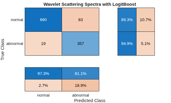
Compute the F1 scores and display the macro-averaged precision, recall, and F1 scores.
PRTableScatSpectra = helperF1heartSounds(testCVScatSpectra.NormalizedValues);
disp(PRTableScatSpectra)
                     Precision    Recall    F1_Score
                     _________    ______    ________
    Abnormal          81.136      94.947       87.5
    Normal             97.32      89.263     93.117
    Macro Average     89.228      92.105     90.309
Using Phase Harmonics
Next, use the phase harmonic method. Setting method="phaseharmonic", replaces the modulus-modulus coefficients of wavelet scattering spectra with wavelet phase harmonics. This means that there are many common features between method="scatteringspectra" and method="phaseharmonic". See the documentation for details and guidance on which method to choose. Depending on the network configuration, using method="phaseharmonic" can result in a significant reduction in the number of coefficients. In this example, the number of coefficients per signal is reduced from 10,000 to 674 for Method="scatteringspectra" and down to 290 using Method="phaseharmonic". However, there is usually an increase in computation time. Use the same wavelet scattering network and input normalization used in the scattering spectra computation.
[scatPHTrain,phTable] = scatteringSpectra(tsn,trainData,Method="phaseharmonic",...
    OutputMode="realimag", ...
    InputNormalization="std");
scatPHTest = scatteringSpectra(tsn,testData,Method="phaseharmonic", ...
    OutputMode="realimag", ...
    InputNormalization="std");
Use the same LogitBoost ensemble described in Training LogitBoost Ensemble.
lboostmdlPH = fitcensemble(scatPHTrain', trainLabels, ...
    Method="LogitBoost", ...
    NumLearningCycles=500, ...
    Learners=T, ...
    LearnRate=0.05, ...
    ClassNames=["abnormal","normal"], ...
    Cost=[0, 2; 1, 0], ...
    Resample="on", ...
    Replace="off", ...
    Fresample=0.8);
Test LogitBoost Ensemble model with Phase Harmonics
Compute the test features and predict the class of the test data.
predTestLabelsPH = categorical(predict(lboostmdlPH,scatPHTest'));
testAccuracy = sum(predTestLabelsPH==testLabels)/numel(testLabels)*100;
fprintf('Test Accuracy is %2.2f percent\n',testAccuracy);
Test Accuracy is 91.56 percent
Obtain the confusion chart with precision and recall values, compute the F1 scores and display the results.
testCVScatPH = confusionchart(testLabels, ...
predTestLabelsPH, ...
RowSummary="row-normalized",ColumnSummary="column-normalized");
title("Wavelet Scattering Phase Harmonics with LogitBoost")

Compute the F1 scores and display the macro-averaged precision, recall, and F1 scores.
PRTablePH = helperF1heartSounds(testCVScatPH.NormalizedValues);
disp(PRTablePH)
                     Precision    Recall    F1_Score
                     _________    ______    ________
    Abnormal          81.922      95.213     88.069
    Normal            97.472       89.78     93.468
    Macro Average     89.697      92.496     90.768
Of the 1149 test records, approximately 91.5% are correctly classified as "Normal" or "Abnormal". Of the 773 normal PCG recordings in the test set, 694 are correctly classified. Of the 376 abnormal recordings in the test set, 358 are correctly classified.
Summary
Both models perform quite well on the held-out test set. The macro-averaged F1 scores are nearly identical. However, the use of phase harmonics has resulted in a reduction in the number of features by a factor of 2.3. Accordingly, you have nearly identical precision, recall, and F1 metrics with less than 1/2 the features.
Both models detect roughly 96% of the actual abnormal cases (high recall), which is exactly what the asymmetric cost matrix was designed to encourage. The tradeoff is lower precision (approximately 81%), meaning roughly 1 in 5 samples flagged as abnormal are actually normal (false positives). Again, this can be adjusted by changing the penalties in the cost matrix.
Of course with the normal class, the pattern is reversed. Precision is very high (97-98%), so when the model designates a waveform as "normal," it is almost always right. But recall is lower (88-89%), meaning about 11% of truly normal cases are misclassified as abnormal. Again, this is the direct consequence of the cost matrix pushing the decision boundary toward flagging more abnormal cases. Due to the stochastic nature of the training, rerunning the example may change the results slightly, but the general outcomes will remain the same.
The macro-averaged F1 scores of 90% plus indicate good balanced performance across the classes, suggesting the ensemble's regularization strategy (slow learning rate, feature/observation subsampling, and shallow trees) is generalizing well.
Scattering Spectra or Phase Harmonics?
The practical takeaway is that both feature sets perform equally well. The differences are well within the range of normal statistical variation. If you ran cross-validation or repeated hold-out splits, you would likely see fluctuations of this magnitude between folds. Substituting the phase harmonics for the modulus-modulus coefficients does not result in a significant difference. However, you can use other criteria to make an informed choice between them such as: the smaller feature set for the phase harmonics, or the slightly higher computational cost of the phase harmonics over the scattering spectra.
Comparison with Full Scattering Transform
The full scattering transform used in Wavelet Time Scattering Classification of Phonocardiogram Data performs slightly better than the scattering spectra-phase harmonic approach shown here. The following table summarizes the macro-averaged precision, recall, and F1 score metrics across the three approaches.
Method | Precision | Recall | F1 Score |
Scattering Transform with Majority Vote |
| 93.431 | 91.387 |
Scattering Spectra | 89.228 | 92.105 | 90.309 |
Phase Harmonics | 89.697 | 92.496 | 90.768 |
Given the stochastic nature of training machine learning algorithms and the different techniques used in each case, these results are very likely within the range of expected statistical variation. One clear advantage of the scattering spectra-phase harmonic approach is interpretability. With the scattering spectra-phase harmonic approach, the coefficients are always interpretable as correlations between scale-aligned wavelet coefficients. On the other hand, the majority vote method employed with the full scattering transform is more difficult to interpret because it obtains one class prediction for every scattering coefficient across all the paths. That approach is sensitive to the OversamplingFactor in the scattering transform. On the other hand, the scattering spectra method reduces each correlation to a scalar irrespective of the OversamplingFactor. One potential disadvantage of the scattering spectra-phase harmonic approach is the growth in the number of coefficients as the quality factor increases, while the number of paths in the scattering transform grows much more slowly as the quality factor increases. See the documentation for more detail on the differences between the scattering transform and the scattering spectra-phase harmonic approach.
References
Goldberger, A. L., L. A. N. Amaral, L. Glass, J. M. Hausdorff, P. Ch. Ivanov, R. G. Mark, J. E. Mietus, G. B. Moody, C.-K. Peng, and H. E. Stanley. "PhysioBank, PhysioToolkit, and PhysioNet: Components of a New Research Resource for Complex Physiologic Signals". Circulation. Vol. 101, No. 23, 13 June 2000, pp. e215-e220. https://circ.ahajournals.org/content/101/23/e215.full.
Lempereur, Etienne, Nathanaël Cuvelle–Magar, Florentin Coeurdoux, Stéphane Mallat, and Eric Vanden-Eijnden. 2026. "MGD: Moment Guided Diffusion for Maximum Entropy Generation." arXiv preprint. https://arxiv.org/abs/2602.17211.
Liu et al. "An open access database for the evaluation of heart sound algorithms". Physiological Measurement. Vol. 37, No. 12, 21 November 2016, pp. 2181-2213. https://www.ncbi.nlm.nih.gov/pubmed/27869105.
Mallat, Stephane, Sixin Zhang, and Gaspar Rochette. 2019. "Phase harmonic Correlations and Convolutional Neural Networks". Journal of Information and Inference, 721-747, https://doi.org/10.1093/imaiai/iaz019.
Morel, Rudy, Gaspar Rochette, Roberto Leonarduzzi, Jean-Philippe Bouchaud, and Stéphane Mallat. 2024. "Scale Dependencies and Self-Similar Models with Wavelet Scattering Spectra." Applied and Computational Harmonic Analysis, November, 101724–24. https://doi.org/10.1016/j.acha.2024.101724.
Regaldo-Saint Blanchard, Bruno, Erwan Allys, Constant AuClair, Francois Boulanger, Michael Eickenburg, Francois Levrier, Leo Vacher, and Sixin Zhang. 2023. "Generative Models of Multi-channel Data from a Single Example - Application to Dust Emission." The Astrophysical Journal 943 (2023): 9. https://doi.org/10.3847/1538-4357/aca538.
Supporting Functions
function PRTable = helperF1heartSounds(confmat)
% This function is only in support of Scattering Spectra and
% Wavelet Phase Harmonics with Phonocardiogram Data It may change or be
% removed in a future release.
precisionAB = confmat(2,2)/sum(confmat(:,2))*100;
precisionNR = confmat(1,1)/sum(confmat(:,1))*100 ;
recallAB = confmat(2,2)/sum(confmat(2,:))*100;
recallNR = confmat(1,1)/sum(confmat(1,:))*100;
F1AB = 2*(precisionAB*recallAB)/(precisionAB+recallAB);
F1NR = 2*(precisionNR*recallNR)/(precisionNR+recallNR);
MacroAverages = mean(cat(2,[precisionAB; precisionNR],...
    [recallAB;recallNR], [F1AB;F1NR]));
% Construct a MATLAB Table to display the results.
PRTable = array2table([precisionAB recallAB F1AB;...
    precisionNR recallNR F1NR; ...
    MacroAverages],...
    VariableNames = ["Precision","Recall","F1_Score"],...
    RowNames = ["Abnormal","Normal","Macro Average"]);
end

