Tunable Q-factor Wavelet Transform
The Q-factor of a wavelet transform is the ratio of the center frequency to the bandwidth of the filters used in the transform. The tunable Q-factor wavelet transform (TQWT) is a technique that creates a wavelet multiresolution analysis (MRA) with a user-specified Q-factor. The TQWT provides perfect reconstruction of the signal. The TQWT coefficients partition the energy of the signal into subbands.
The TQWT was developed by Selesnick [1]. The algorithm uses
filters specified directly in the frequency domain and can be efficiently implemented using
FFTs. The wavelets satisfy the Parseval frame property. The TQWT is defined by two
variables: the Q-factor and the redundancy, also known as the oversampling rate. To obtain
wavelets well-localized in time, Selesnick recommends a redundancy r ≥ 3.
As implemented, the tqwt,
itqwt, and
tqwtmra
functions use the fixed redundancy r = 3.
Discrete wavelet transforms (DWT) use the fixed Q-factor of √2. The value √2 follows from the definition of the MRA leading to an orthogonal wavelet transform. However, depending on the data, other Q-factors may be desirable. Higher Q-factors result in more narrow filters, which are better for analyzing oscillatory signals. To analyze signals with transient components, lower Q-factors are more appropriate.
Frequency-Domain Scaling
A fundamental component of the TQWT is scaling in the frequency domain:
lowpass scaling — frequency-domain scaling that preserves low-frequency content
highpass scaling — frequency-domain scaling that preserves high-frequency content
When you scale a signal x(n) that is sampled at a rate fs in the frequency domain, you change the sample rate of the output signal y(n). If X(ω) and Y(ω) are the discrete-time Fourier transforms of x(n) and y(n), respectively, and 0 < α < 1, lowpass scaling by α (LPS α) in the frequency domain is defined as
For lowpass scaling, the output signal is sampled at α·fs. If 0 < β ≤ 1, highpass scaling by β (HPS β) is defined as
For highpass scaling, the output signal is sampled at β·fs. Similar definitions exist for the cases α > 1 and β > 1.
TQWT Algorithm
The TQWT algorithm is implemented as a two-channel filter bank. In the analysis direction, the lowpass subband v0(n) has a sample rate of α·fs, and the highpass subband v1(n) has a sample rate of β·fs. We say that the filter bank is oversampled by a factor of α + β.

The lowpass and highpass filters, H0(ω) and H1(ω) respectively, satisfy
and
In the TQWT algorithm, the analysis filter bank is applied iteratively to the lowpass output of the previous iteration. The sample rate of the highpass output at kth iteration is β·αk-1·fs, where fs is the sample rate of the original input signal. To ensure perfect reconstruction and well-localized (in time) wavelets, the TQWT algorithm requires that α and β satisfy α + β > 1.
Redundancy and Q-factor
In the TQWT, and . As stated above, the sample rate at the kth iteration is , where is the original sample rate. As the iterations continue, the sample rate converges to The quantity is the redundancy of the TQWT. The support of the frequency response of the kth iteration of the highpass filter, , is in the interval . The center frequency of the highpass filter is approximately equal to the average of the frequencies at the ends of the interval: . The bandwidth is the length of the interval: . The Q-factor is .
To illustrate how the redundancy and Q-factor affect the transition bands of the lowpass and highpass filters, and respectively, use the helper function helperPlotLowAndHighpassFilters to plot the frequency responses of the filters for different redundancy and Q-factor values. Source code for the helper function is in the same directory as this example file. The helper function uses filters based on the Daubechies frequency response: for . For more information, see [1].
qualityFactor =2; redundancy =
3; helperPlotLowAndHighpassFilters(qualityFactor,redundancy)

As implemented, the tqwt, itqwt, and tqwtmra functions use a fixed redundancy of 3. To see how the Q-factor affects the wavelet, use the helper function helperPlotQfactorWavelet to plot the wavelet in the time domain for different integer values of the Q-factor. Observe that for a fixed Q-factor, the wavelet support decreases as the scale grows finer. For analyzing oscillatory signals, higher Q-factors are better.
qf =1; scale =
8; helperPlotQfactorWavelet(qf,scale)
9

Example: MRA of Audio Signal
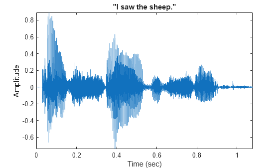
Load and plot a recording of a female speaker saying "I saw the sheep". The sample rate is 22,050 Hz.
load wavsheep
plot(tsh,sheep)
axis tight
title('"I saw the sheep."')
xlabel("Time (sec)")
ylabel("Amplitude")
Obtain the TQWT using the default quality factor of 1.
[wt1,info1] = tqwt(sheep);
The output info1 is a structure array that contains information about the TQWT. The field CenterFrequencies contains the normalized center frequencies (cycles/sample) of the wavelet subbands. The field Bandwidths contains the approximate bandwidths of the wavelet subbands in normalized frequency. For every subband, confirm that the ratio of the center frequency to the bandwidth is equal to the quality factor.
ratios = info1.CenterFrequencies./info1.Bandwidths;
[min(ratios) max(ratios)]
ans = 1×2

     1     1
Display , the highpass scaling factor, and , the lowpass scaling factor. As implemented, the functions tqwt, itqwt, and tqwtmra use the redundancy factor . Confirm that the scaling factors satisfy the relation .
[info1.Beta info1.Alpha]
ans = 1×2

    1.0000    0.6667
r = info1.Beta/(1-info1.Alpha)
r =
3.0000
Identify the subbands that contain at least 15% of the total energy. Note that the last element of wt1 contains the lowpass subband coefficients. Confirm the sum of the percentages equals 100.
EnergyBySubband = cellfun(@(x)norm(x,2)^2,wt1)./norm(sheep,2)^2*100;
idx15 = EnergyBySubband >= 15;
bar(EnergyBySubband)
title("Percent Energy By Subband")
xlabel("Subband")
ylabel("Percent Energy")
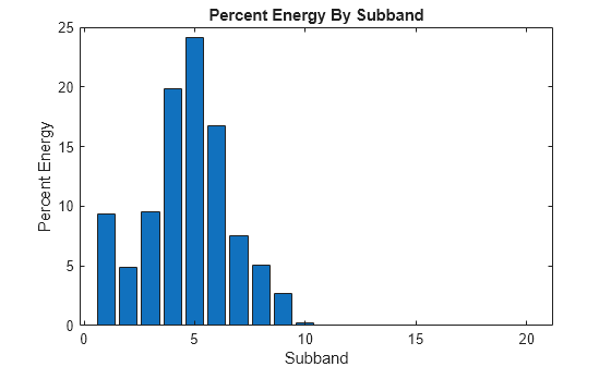
sum(EnergyBySubband)
ans =
100.0000
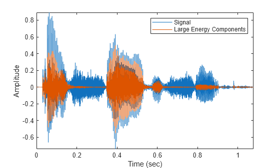
Obtain a multiresolution analysis and sum those MRA components corresponding to previously identified subbands.
mra = tqwtmra(wt1,length(sheep));
ts = sum(mra(idx15,:));
plot(tsh,[sheep ts'])
axis tight
legend("Signal","Large Energy Components")
xlabel("Time (sec)")
ylabel("Amplitude")
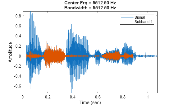
Plot the first subband. Observe that this subband contains frequency content of the words "saw" and "sheep".
mra = tqwtmra(wt1,length(sheep));
str = sprintf("Center Frq = %.2f Hz\nBandwidth = %.2f Hz",...
    fs*info1.CenterFrequencies(1),fs*info1.Bandwidths(1));
plot(tsh,sheep)
hold on
plot(tsh,mra(1,:))
hold off
axis tight
title(str)
legend("Signal","Subband 1")
xlabel("Time (sec)")
ylabel("Amplitude")
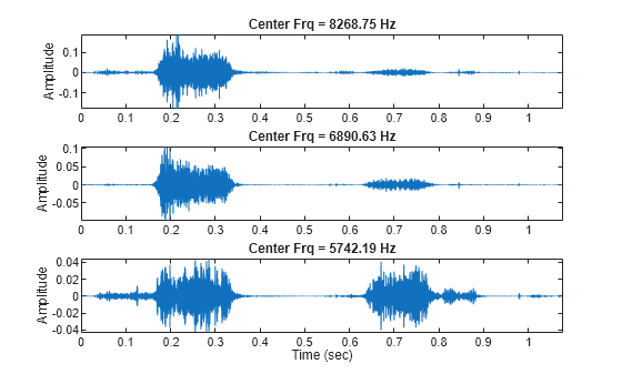
To obtain a finer look of the first subband, obtain a second TQWT of the signal using a quality factor of 3. Inspect the center frequencies, in hertz, of the first five subbands.
[wt3,info3] = tqwt(sheep,QualityFactor=3);
fs*info3.CenterFrequencies(1:5)
ans = 1×5
103 ×

    8.2688    6.8906    5.7422    4.7852    3.9876
The center frequencies of the first three subbands are higher than the center frequency of the first subband of the first TQWT. Obtain the MRA of the signal using a quality factor of 3, and plot the first three MRA components. Compare the frequency content of the words "saw" and "sheep" in the three subbands. Most of the energy in the first subband comes from the word "saw".
mra = tqwtmra(wt3,length(sheep),QualityFactor=3);
for k=1:3
    str = sprintf("Center Frq = %.2f Hz",fs*info3.CenterFrequencies(k));
    subplot(3,1,k)
    plot(tsh,mra(k,:))
    axis tight
    title(str)
    ylabel("Amplitude")
end
xlabel("Time (sec)")
Plot the percentage of total energy each subband contains when quality factor is 3. Confirm the sum of the percentages equals 100.
EnergyBySubband = cellfun(@(x)norm(x,2)^2,wt3)./norm(sheep,2)^2*100;
figure
bar(EnergyBySubband)
title("Percent Energy By Subband")
xlabel("Subband")
ylabel("Percent Energy")
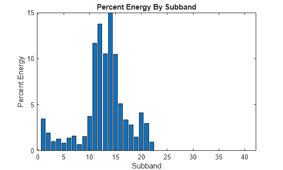
sum(EnergyBySubband)
ans =
100.0000
References
[1] Selesnick, Ivan W. “Wavelet Transform With Tunable Q-Factor.” IEEE Transactions on Signal Processing 59, no. 8 (August 2011): 3560–75. https://doi.org/10.1109/TSP.2011.2143711.
[2] Daubechies, Ingrid. Ten Lectures on Wavelets. CBMS-NSF Regional Conference Series in Applied Mathematics 61. Philadelphia, Pa: Society for Industrial and Applied Mathematics, 1992.