36846
Results for
Yes, some readers might now argue that I used roughness in a crazy way in my last post, in my approach to finding a large twin prime pair. That is, I deliberately constructed a family of integers that were known to be a-priori rough. But, suppose I gave you some large, rather arbitrarily constructed number, and asked you to tell me if it is prime? For example, to pull a number out of my hat, consider
P = sym(2)^122397 + 65;
floor(vpa(log10(P) + 1))
36846 decimal digits is pretty large. And in fact, large enough that sym/isprime in R2024b will literally choke on it. But is it prime? Can we efficiently learn if it is at least not prime?
A nice way to learn the roughness of even a very large number like this is to use GCD.
gcd(P,prod(sym(primes(10000))))
If the greatest common divisor between P and prod(sym(primes(10000))) is 1, then P is NOT divisible by any small prime from that set, since they have no common divisors. And so we can learn that P is indeed fairly rough, 10000-rough in fact. That means P is more likely to be prime than most other large integers in that domain.
gcd(P,prod(sym(primes(100000))))
However, this rather efficiently tells us that in fact, P is not prime, as it has a common factor with some integer greater than 1, and less then 1e5.
I suppose you might think this is nothing different from doing trial divides, or using the mod function. But GCD is a much faster way to solve the problem. As a test, I timed the two.
timeit(@() gcd(P,prod(sym(primes(100000)))))
timeit(@() any(mod(P,primes(100000)) == 0))
Even worse, in the first test, much if not most of that time is spent in merely computing the product of those primes.
pprod = prod(sym(primes(100000)));
timeit(@() gcd(P,pprod))
So even though pprod is itself a huge number, with over 43000 decimal digits, we can use it quite efficiently, especially if you precompute that product if you will do this often.
How might I use roughness, if my goal was to find the next larger prime beyond 2^122397? I'll look fairly deeply, looking only for 1e7-rough numbers, because these numbers are pretty seriously large. Any direct test for primality will take some serious time to perform.
pprod = prod(sym(primes(10000000)));
find(1 == gcd(sym(2)^122397 + (1:2:199),pprod))*2 - 1
2^122397 plus any one of those numbers is known to be 1e7-rough, and therefore very possibly prime. A direct test at this point would surely take hours and I don't want to wait that long. So I'll back off just a little to identify the next prime that follows 2^10000. Even that will take some CPU time.
What is the next prime that follows 2^10000? In this case, the number has a little over 3000 decimal digits. But, even with pprod set at the product of primes less than 1e7, only a few seconds were needed to identify many numbers that are 1e7-rough.
P10000 = sym(2)^10000;
k = find(1 == gcd(P10000 + (1:2:1999),pprod))*2 - 1
k =
Columns 1 through 8
15 51 63 85 165 171 177 183
Columns 9 through 16
253 267 273 295 315 421 427 451
Columns 17 through 24
511 531 567 601 603 675 687 717
Columns 25 through 32
723 735 763 771 783 793 795 823
Columns 33 through 40
837 853 865 885 925 955 997 1005
Columns 41 through 48
1017 1023 1045 1051 1071 1075 1095 1107
Columns 49 through 56
1261 1285 1287 1305 1371 1387 1417 1497
Columns 57 through 64
1507 1581 1591 1593 1681 1683 1705 1771
Columns 65 through 69
1773 1831 1837 1911 1917
Among the 1000 odd numbers immediately following 2^10000, there are exactly 69 that are 1e7-rough. Every other odd number in that sequence is now known to be composite, and even though we don't know the full factorization of those 931 composite numbers, we don't care in the context as they are not prime. I would next apply a stronger test for primality to only those few candidates which are known to be rough. Eventually after an extensive search, we would learn the next prime succeeding 2^10000 is 2^10000+13425.
In my next post, I show how to use MOD, and all the cores in your CPU to test for roughness.
How can we use roughness in an effective context to identify large primes? I can quickly think of quite a few examples where we might do so. Again, remember I will be looking for primes with not just hundreds of decimal digits, or even only a few thousand digits. The eventual target is higher than that. Forget about targets for now though, as this is a journey, and what matters in this journey is what we may learn along the way.
I think the most obvious way to employ roughness is in a search for twin primes. Though not yet proven, the twin prime conjecture:
If it is true, it tells us there are infinitely many twin prime pairs. A twin prime pair is two integers with a separation of 2, such that both of them are prime. We can find quite a few of them at first, as we have {3,5}, {5,7}, {11,13}, etc. But there is only ONE pair of integers with a spacing of 1, such that both of them are prime. That is the pair {2,3}. And since primes are less and less common as we go further out, possibly there are only a finite number of twins with a spacing of exactly 2? Anyway, while I'm fairly sure the twin prime conjecture will one day be shown to be true, it can still be interesting to search for larger and larger twin prime pairs. The largest such known pair at the moment is
2996863034895*2^1290000 +/- 1
This is a pair with 388342 decimal digits. And while seriously large, it is still in range of large integers we can work with in MATLAB, though certainly not in double precision. In my own personal work on my own computer, I've done prime testing on integers (in MATLAB) with considerably more than 100,000 decimal digits.
But, again you may ask, just how does roughness help us here? In fact, this application of roughness is not new with me. You might want to read about tools like NewPGen {https://t5k.org/programs/NewPGen/} which sieves out numbers known to be composite, before any direct tests for primality are performed.
Before we even try to talk about numbers with thousands or hundreds of thousands of decimal digits, look at 6=2*3. You might observe
isprime([-1,1] + 6)
shows that both 5 and 7 are prime. This should not be a surprise, but think about what happens, about why it generated a twin prime pair. 6 is divisible by both 2 and 3, so neither 5 or 7 can possibly be divisible by either small prime as they are one more or one less than a multiple of both 2 and 3. We can try this again, pushing the limits just a bit.
isprime([-1,1] + 2*3*5)
That is again interesting. 30=2*3*5 is evenly divisible by 2, 3, and 5. The result is both 29 and 31 are prime, because adding 1 or subtracting 1 from a multiple of 2, 3, or 5 will always result in a number that is not divisible by any of those small primes. The next larger prime after 5 is 7, but it cannot be a factor of 29 or 31, since it is greater than both sqrt(29) and sqrt(31).
We have quite efficiently found another twin prime pair. Can we take this a step further? 210=2*3*5*7 is the smallest such highly composite number that is divisible by all primes up to 7. Can we use the same trick once more?
isprime([-1,1] + 2*3*5*7)
And here the trick fails, because 209=11*19 is not in fact prime. However, can we use the large twin prime trick we saw before? Consider numbers of the form [-1,1]+a*210, where a is itself some small integer?
a = 2;
isprime([-1,1] + a*2*3*5*7)
I did not need to look far, only out to a=2, because both 419 and 421 are prime. You might argue we have formed a twin prime "factory", of sorts. Next, I'll go out as far as the product of all primes not exceeding 60. This is a number with 22 decimal digits, already too large to represent as a double, or even as uint64.
prod(sym(primes(60)))
a = find(all(isprime([-1;1] + prod(sym(primes(60)))*(1:100)),1))
That easily identifies 3 such twin prime pairs, each of which has roughly 23 decimal digits, each of which have the form a*1922760350154212639070+/-1. The twin prime factory is still working well. Going further out to integers with 37 decimal digits, we can easily find two more such pairs that employ the product of all primes not exceeding 100.
prod(sym(primes(100)))
a = find(all(isprime([-1;1] + prod(sym(primes(100)))*(1:100)),1))
This is in fact an efficient way of identifying large twin prime pairs, because it chooses a massively composite number as the product of many distinct small primes. Adding or subtracting 1 from such a number will result always in a rough number, not divisible by any of the primes employed. With a little more CPU time expended, now working with numbers with over 1000 decimal digits, I will claim this next pair forms a twin prime pair, and is the smallest such pair we can generate in this way from the product of the primes not exceeding 2500.
isprime(7826*prod(sym(primes(2500))) + [-1 1])
ans =
logical
1
Unfortunately, 1000 decimal digits is at or near the limit of what the sym/isprime tool can do for us. It does beg the question, asking if there are alternatives to the sym/isprime tool, as an isProbablePrime test, usually based on Miller-Rabin is often employed. But this is gist for yet another set of posts.
Anyway, I've done a search for primes of the form
a*prod(sym(primes(10000))) +/- 1
having gone out as far as a = 600000, with no success as of yet. (My estimate is I will find a pair by the time I get near 5e6 for a.) Anyway, if others can find a better way to search for large twin primes in MATLAB, or if you know of a larger twin prime pair of this extended form, feel free to chime in.
My next post shows how to use GCD in a very nice way to identify roughness, on a large scale.
What is a rough number? What can they be used for? Today I'll take you down a journey into the land of prime numbers (in MATLAB). But remember that a journey is not always about your destination, but about what you learn along the way. And so, while this will be all about primes, and specifically large primes, before we get there we need some background. That will start with rough numbers.
Rough numbers are what I would describe as wannabe primes. Almost primes, and even sometimes prime, but often not prime. They could've been prime, but may not quite make it to the top. (If you are thinking of Marlon Brando here, telling us he "could've been a contender", you are on the right track.)
Mathematically, we could call a number k-rough if it is evenly divisible by no prime smaller than k. (Some authors will use the term k-rough to denote a number where the smallest prime factor is GREATER than k. The difference here is a minor one, and inconsequential for my purposes.) And there are also smooth numbers, numerical antagonists to the rough ones, those numbers with only small prime factors. They are not relevant to the topic today, even though smooth numbers are terribly valuable tools in mathematics. Please forward my apologies to the smooth numbers.
Have you seen rough numbers in use before? Probably so, at least if you ever learned about the sieve of Eratosthenes for prime numbers, though probably the concept of roughness was never explicitly discussed at the time. The sieve is simple. Suppose you wanted a list of all primes less than 100? (Without using the primes function itself.)
% simple sieve of Eratosthenes
Nmax = 100;
N = true(1,Nmax); % A boolean vector which when done, will indicate primes
N(1) = false; % 1 is not a prime by definition
nextP = find(N,1,'first'); % the first prime is 2
while nextP <= sqrt(Nmax)
% flag multiples of nextP as not prime
N(nextP*nextP:nextP:end) = false;
% find the first element after nextP that remains true
nextP = nextP + find(N(nextP+1:end),1,'first');
end
primeList = find(N)
Indeed, that is the set of all 25 primes not exceeding 100. If you think about how the sieve worked, it first found 2 is prime. Then it discarded all integer multiples of 2. The first element after 2 that remains as true is 3. 3 is of course the second prime. At each pass through the loop, the true elements that remain correspond to numbers which are becoming more and more rough. By the time we have eliminated all multiples of 2, 3, 5, and finally 7, everything else that remains below 100 must be prime! The next prime on the list we would find is 11, but we have already removed all multiples of 11 that do not exceed 100, since 11^2=121. For example, 77 is 11*7, but we already removed it, because 77 is a multiple of 7.
Such a simple sieve to find primes is great for small primes. However is not remotely useful in terms of finding primes with many thousands or even millions of decimal digits. And that is where I want to go, eventually. So how might we use roughness in a useful way? You can think of roughness as a way to increase the relative density of primes. That is, all primes are rough numbers. In fact, they are maximally rough. But not all rough numbers are primes. We might think of roughness as a necessary, but not sufficient condition to be prime.
How many primes lie in the interval [1e6,2e6]?
numel(primes(2e6)) - numel(primes(1e6))
There are 70435 primes greater than 1e6, but less than 2e6. Given there are 1 million natural numbers in that set, roughly 7% of those numbers were prime. Next, how many 100-rough numbers lie in that same interval?
N = (1e6:2e6)';
roughInd = all(mod(N,primes(100)) > 0,2);
sum(roughInd)
That is, there are 120571 100-rough numbers in that interval, but all those 70435 primes form a subset of the 100-rough numbers. What does this tell us? Of the 1 million numbers in that interval, approximately 12% of them were 100-rough, but 58% of the rough set were prime.
The point being, if we can efficiently identify a number as being rough, then we can substantially increase the chance it is also prime. Roughness in this sense is a prime densifier. (Is that even a word? It is now.) If we can reduce the number of times we need to perform an explicit isprime test, that will gain greatly because a direct test for primality is often quite costly in CPU time, at least on really large numbers.
In my next post, I'll show some ways we can employ rough numbers to look for some large primes.
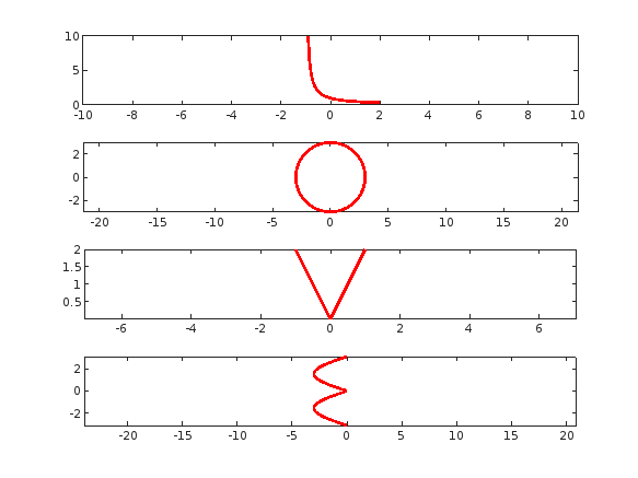
tiledlayout(4,1);
% Plot "L" (y = 1/(x+1), for x > -1)
x = linspace(-0.9, 2, 100); % Avoid x = -1 (undefined)
y =1 ./ (x+1) ;
nexttile;
plot(x, y, 'r', 'LineWidth', 2);
xlim([-10,10])
% Plot "O" (x^2 + y^2 = 9)
theta = linspace(0, 2*pi, 100);
x = 3 * cos(theta);
y = 3 * sin(theta);
nexttile;
plot(x, y, 'r', 'LineWidth', 2);
axis equal;
% Plot "V" (y = -2|x|)
x = linspace(-1, 1, 100);
y = 2 * abs(x);
nexttile;
plot(x, y, 'r', 'LineWidth', 2);
axis equal;
% Plot "E" (x = -3 |sin(y)|)
y = linspace(-pi, pi, 100);
x = -3 * abs(sin(y));
nexttile;
plot(x, y, 'r', 'LineWidth', 2);
axis equal;
Check out the result of "emoji matrix" multiplication below.
- vector multiply vector:
a = ["😁","😁","😁"]
b = ["😂";
"😂"
"😂"]
c = a*b
d = b*a
- matrix multiply matrix:
matrix1 = [
"😀", "😃";
"😄", "😁"]
matrix2 = [
"😆", "😅";
"😂", "🤣"]
resutl = matrix1*matrix2
enjoy yourself!
Creating data visualizations
79%
Interpreting data visualizations
21%
28 votes
For Valentine's day this year I tried to do something a little more than just the usual 'Here's some MATLAB code that draws a picture of a heart' and focus on how to share MATLAB code. TL;DR, here's my advice
- Put the code on GitHub. (Allows people to access and collaborate on your code)
- Set up 'Open in MATLAB Online' in your GitHub repo (Allows people to easily run it)
I used code by @Zhaoxu Liu / slandarer and others to demonstrate. I think that those two steps are the most impactful in that they get you from zero to one but If I were to offer some more advice for research code it would be
3. Connect the GitHub repo to File Exchange (Allows MATLAB users to easily find it in-product).
4. Get a Digitial Object Identifier (DOI) using something like Zenodo. (Allows people to more easily cite your code)
There is still a lot more you can do of course but if everyone did this for any MATLAB code relating to a research paper, we'd be in a better place I think.
Here's the article: On love and research software: Sharing code with your Valentine » The MATLAB Blog - MATLAB & Simulink
What do you think?
Have you ever wanted to search for a community member but didn't know where to start? Or perhaps you knew where to search but couldn't find enough information from the results? You're not alone. Many community users have shared this frustration with us. That's why the community team is excited to introduce the new ‘People’ page to address this need.

What Does the ‘People’ Page Offer?
- Comprehensive User Search: Search for users across different applications seamlessly.
- Detailed User Information: View a list of community members along with additional details such as their join date, rankings, and total contributions.
- Sorting Options: Use the ‘sort by’ filter located below the search bar to organize the list according to your preferences.
- Easy Navigation: Access the Answers, File Exchange, and Cody Leaderboard by clicking the ‘Leaderboards’ button in the upper right corner.
In summary, the ‘People’ page provides a gateway to search for individuals and gain deeper insights into the community.
How Can You Access It?
Navigate to the global menu, click on the ‘More’ link, and you’ll find the ‘People’ option.
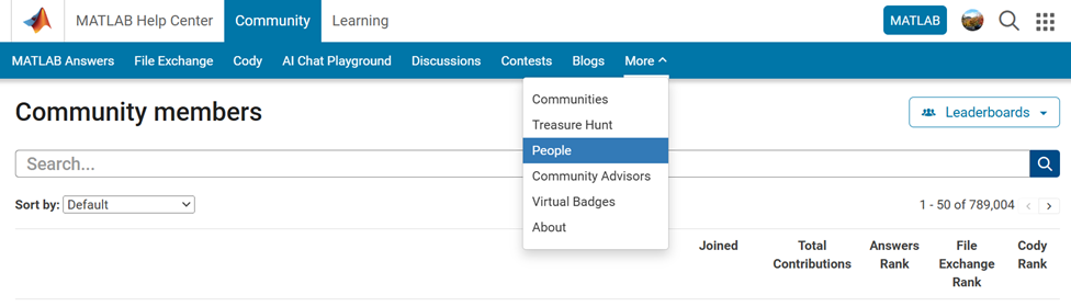
Now you know where to go if you want to search for a user. We encourage you to give it a try and share your feedback with us.
Los invito a conocer el libro "Sistemas dinámicos en contexto: Modelación matemática, simulación, estimación y control con MATLAB", el cual ya está disponible en formato digital.
El libro integra diversos temas de los sistemas dinámicos desde un punto de vista práctico utilizando programas de MATLAB y simulaciones en Simulink y utilizando métodos numéricos (ver enlace). Existe mucho material en el blog del libro con posibilidades para comentarios, propuestas y correcciones. Resalto los casos de estudio
Creo que el libro les puede dar un buen panorama del área con la posibilidad de experimentar de manera interactiva con todo el material de MATLAB disponible en formato Live Script. Lo mejor es que se pueden formular preguntas en el blog y hacer propuestas al autor de ejercicios resueltos.
Son bienvenidos los comentarios, sugerencias y correcciones al texto.
Simulink has been an essential tool for modeling and simulating dynamic systems in MATLAB. With the continuous advancements in AI, automation, and real-time simulation, I’m curious about what the future holds for Simulink.
What improvements or new features do you think Simulink will have in the coming years? Will AI-driven modeling, cloud-based simulation, or improved hardware integration shape the next generation of Simulink?
I got thoroughly nerd-sniped by this xkcd, leading me to wonder if you can use MATLAB to figure out the dice roll for any given (rational) probability. Well, obviously you can. The question is how. Answer: lots of permutation calculations and convolutions.
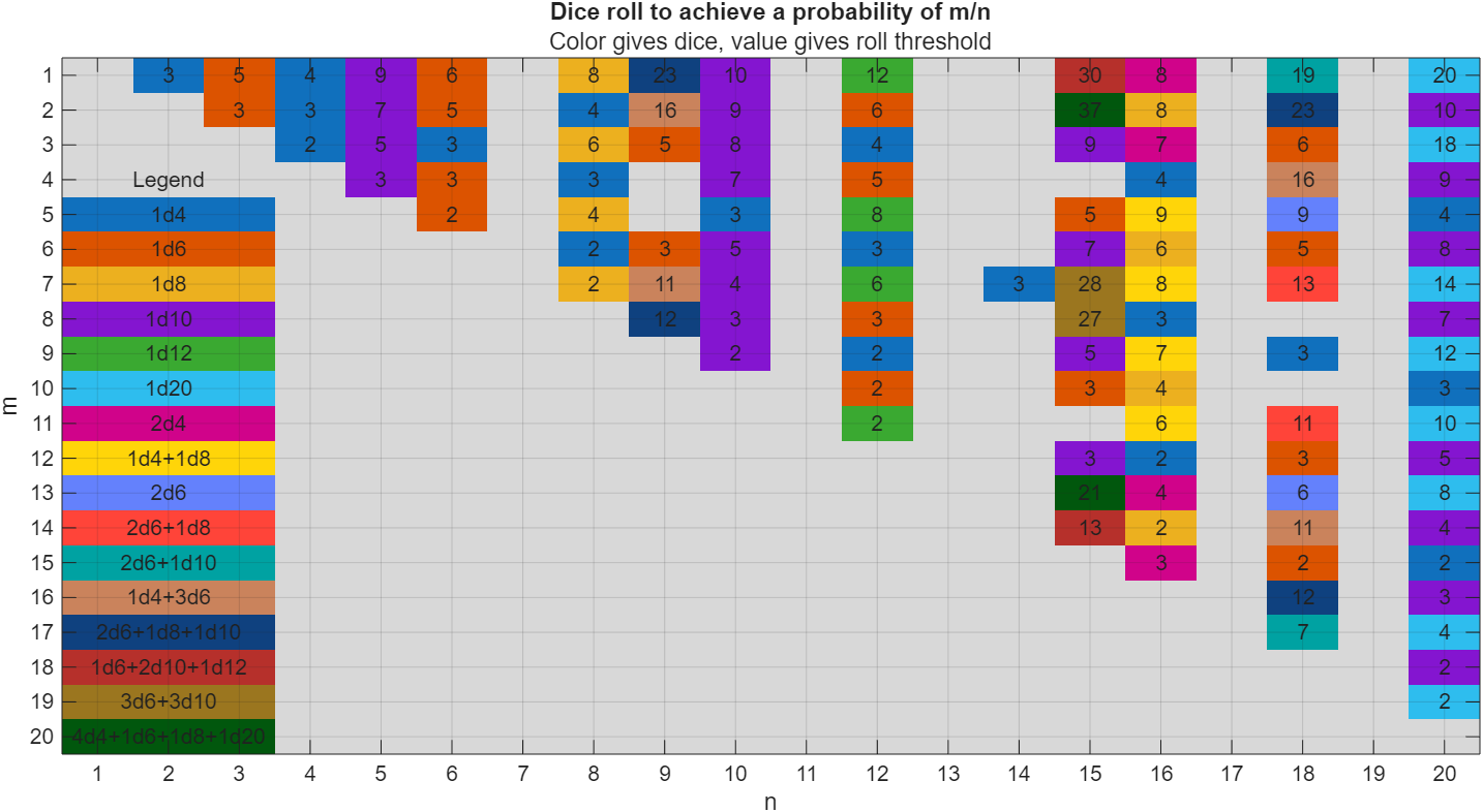
In the original xkcd, the situation described by the player has a probability of 2/9. Looking up the plot, row 2 column 9, shows that you need 16 or greater on (from the legend) 1d4+3d6, just as claimed.
If you missed the bit about convolutions, this is a super-neat trick
[v,c] = dicedist([4 6 6 6]);
bar(v,c)
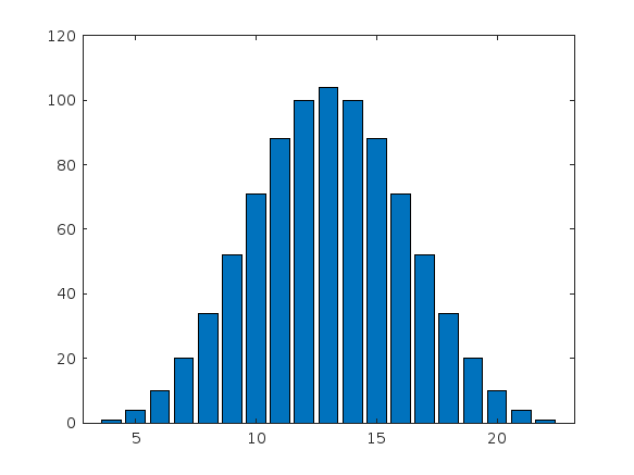
% Probability distribution of dice given by d
function [vals,counts] = dicedist(d)
% d is a vector of number of sides
n = numel(d); % number of dice
% Use convolution to count the number of ways to get each roll value
counts = 1;
for k = 1:n
counts = conv(counts,ones(1,d(k)));
end
% Possible values range from n to sum(d)
maxtot = sum(d);
vals = n:maxtot;
end
The pdist function allows the user to specify the function coding the similarity between rows of matrices (called DISTFUN in the documentation).
With the increasing diffusion of large datasets, techniques to sparsify graphs are increasingly being explored and used in practical applications. It is easy to code one own's DISTFUN such that it returns a sparse vector. Unfortunately, pdist (and pdist2) will return a dense vector in the output, which for very large graphs will cause an out of memory error. The offending code is
(lines 434 etc.)
% Make the return have whichever numeric type the distance function
% returns, or logical.
if islogical(Y)
Y = false(1,n*(n-1)./2);
else % isnumeric
Y = zeros(1,n*(n-1)./2, class(Y));
end
To have pdist return a sparse vector, the only modification that is required is
if islogical(Y)
Y = false(1,n*(n-1)./2);
elseif issparse(Y)
Y = sparse(1,n*(n-1)./2);
else % isnumeric
Y = zeros(1,n*(n-1)./2, class(Y));
end
It is a bit more work to modify squareform to produce a sparse matrix, given a sparse vector produced by the modified pdist. Squareform includes several checks on the inputs, but the core functionality for sparse vectors would be given by something like
% given a sparse vector d returned by pdist, compute a sparse squareform
[~,j,v] = find(d);
[m,n] = pdist_ind2sub(j, nobs);
W = sparse(m, n, v, nobs, nobs);
W = W + W';
Here, pdist_ind2sub is a function that given a set of indices into a vector produced by pdist, returns the corresponding subscripts in a (triangular) matrix. Computing this requires information about the number of observations given to pdist, i.e. what was n in the preceding code. I could not figure out a way to use the function adjacency to accomplish this.
MATLAB FEX(MATLAB File Exchange) should support Markdown syntax for writing. In recent years, many open-source community documentation platforms, such as GitHub, have generally supported Markdown. MATLAB is also gradually improving its support for Markdown syntax. However, when directly uploading files to the MATLAB FEX community and preparing to write an overview, the outdated document format buttons are still present. Even when directly uploading a Markdown document, it cannot be rendered. We hope the community can support Markdown syntax!
BTW,I know that open-source Markdown writing on GitHub and linking to MATLAB FEX is feasible, but this is a workaround. It would be even better if direct native support were available.
I am very pleased to share my book, with coauthors Professor Richard Davis and Associate Professor Sam Toan, titled "Chemical Engineering Analysis and Optimization Using MATLAB" published by Wiley: https://www.wiley.com/en-us/Chemical+Engineering+Analysis+and+Optimization+Using+MATLAB-p-9781394205363
Also in The MathWorks Book Program:
Chemical Engineering Analysis and Optimization Using MATLAB® introduces cutting-edge, highly in-demand skills in computer-aided design and optimization. With a focus on chemical engineering analysis, the book uses the MATLAB platform to develop reader skills in programming, modeling, and more. It provides an overview of some of the most essential tools in modern engineering design.
Chemical Engineering Analysis and Optimization Using MATLAB® readers will also find:
- Case studies for developing specific skills in MATLAB and beyond
- Examples of code both within the text and on a companion website
- End-of-chapter problems with an accompanying solutions manual for instructors
This textbook is ideal for advanced undergraduate and graduate students in chemical engineering and related disciplines, as well as professionals with backgrounds in engineering design.
You've probably heard about the DeepSeek AI models by now. Did you know you can run them on your own machine (assuming its powerful enough) and interact with them on MATLAB?
In my latest blog post, I install and run one of the smaller models and start playing with it using MATLAB.
Larger models wouldn't be any different to use assuming you have a big enough machine...and for the largest models you'll need a HUGE machine!
Even tiny models, like the 1.5 billion parameter one I demonstrate in the blog post, can be used to demonstrate and teach things about LLM-based technologies.
Have a play. Let me know what you think.
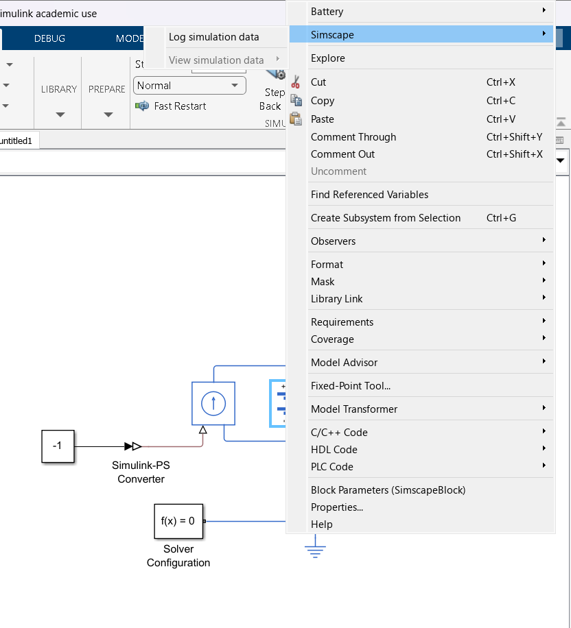
ı m tryna prepare a battery simulation with simulink but when ı push right click on "battery-table based" , and then ı go simscape button, and ı just only see "log simulation data" . Have you any reccomend for this problem? It s probably an easy solution, but ı can't
Too small
22%
Just right
38%
Too large
40%
2648 votes
In one of my MATLAB projects, I want to add a button to an existing axes toolbar. The function for doing this is axtoolbarbtn:
axtoolbarbtn(tb,style,Name=Value)
However, I have found that the existing interfaces and behavior make it quite awkward to accomplish this task.
Here are my observations.
Adding a Button to the Default Axes Toolbar Is Unsupported
plot(1:10)
ax = gca;
tb = ax.Toolbar
Calling axtoolbarbtn on ax results in an error:
>> axtoolbarbtn(tb,"state")
Error using axtoolbarbtn (line 77)
Modifying the default axes toolbar is not supported.
Default Axes Toolbar Can't Be Distinguished from an Empty Toolbar
The Children property of the default axes toolbar is empty. Thus, it appears programmatically to have no buttons, just like an empty toolbar created by axtoolbar.
cla
plot(1:10)
ax = gca;
tb = ax.Toolbar;
tb.Children
ans = 0x0 empty GraphicsPlaceholder array.
tb2 = axtoolbar(ax);
tb2.Children
ans = 0x0 empty GraphicsPlaceholder array.
A Workaround
An empty axes toolbar seems to have no use except to initalize a toolbar before immediately adding buttons to it. Therefore, it seems reasonable to assume that an axes toolbar that appears to be empty is really the default toolbar. While we can't add buttons to the default axes toolbar, we can create a new toolbar that has all the same buttons as the default one, using axtoolbar("default"). And then we can add buttons to the new toolbar.
That observation leads to this workaround:
tb = ax.Toolbar;
if isempty(tb.Children)
% Assume tb is the default axes toolbar. Recreate
% it with the default buttons so that we can add a new
% button.
tb = axtoolbar(ax,"default");
end
btn = axtoolbarbtn(tb);
% Then set up the button as desired (icon, callback,
% etc.) by setting its properties.
As workarounds go, it's not horrible. It just seems a shame to have to delete and then recreate a toolbar just to be able to add a button to it.
The worst part about the workaround is that it is so not obvious. It took me a long time of experimentation to figure it out, including briefly giving it up as seemingly impossible.
The documentation for axtoolbarbtn avoids the issue. The most obvious example to write for axtoolbarbtn would be the first thing every user of it will try: add a toolbar button to the toolbar that gets created automatically in every call to plot. The doc page doesn't include that example, of course, because it wouldn't work.
My Request
I like the axes toolbar concept and the axes interactivity that it promotes, and I think the programming interface design is mostly effective. My request to MathWorks is to modify this interface to smooth out the behavior discontinuity of the default axes toolbar, with an eye towards satisfying (and documenting) the general use case that I've described here.
One possible function design solution is to make the default axes toolbar look and behave like the toolbar created by axtoolbar("default"), so that it has Children and so it is modifiable.
I am curious as to how my goal can be accomplished in Matlab.
The present APP called "Matching Network Designer" works quite well, but it is limited to a single section of a "PI", a "TEE", or an "L" topology circuit.
This limits the bandwidth capability of the APP when the intended use is to create an amplifier design intended for wider bandwidth projects.
I am requesting that a "Broadband Matching Network Designer" APP be developed by you, the MathWorks support team.
One suggestion from me is to be able to cascade a second section (or "pole") to the first.
Then the resulting topology would be capable of achieving that wider bandwidth of the microwave amplifier project where it would be later used with the transistor output and input matching networks.
Instead of limiting the APP to a single frequency, the entire s parameter file would be used as an input.
The APP would convert the polar s parameters to rectangular scaler complex impedances that you already use.
At that point, having started out with the first initial center frequency, the other frequencies both greater than and less than the center would come into use by an optimization of the circuit elements.
I'm hoping that you will be able to take on this project.
I can include an attachment of such a Matching Network Designer APP that you presently have if you like.
That network is centered at 10 GHz.
Kimberly Renee Alvarez.
310-367-5768
Dears,
I am running a MS-DSGE model using RISE toolbox. I want to add a fiscal shock and examine its effect on output, price...
%fiscal shock
shock_type = {'eps_G'};
%here is my variable list of a cell array of character variables and not a struct.
var_list={'log_y','C','pi_ann','B_nominal','B','sp','i_ann','r_real_ann','P'};
% EXOGENOUS SWITCHING
myirfs1=irf(m1,'irf_periods',24,'irf_shock_sign',1);
myirfs1 = struct()
myirfs1.eps_CP = struct();
myirfs1.eps_G = struct();
myirfs1.eps_T = struct();
myirfs1.eps_a = struct();
myirfs1.eps_nu = struct();
myirfs1.eps_z = struct();
var_aux = {'log_y','C','pi_ann','B_nominal','B','sp','i_ann','r_real_ann','P'};
var_aux3 = {'eps_G_log_y','eps_G_C','eps_G_pi_ann','eps_G_B_nominal','eps_G_B','eps_G_sp','eps_G_i_ann','eps_G_r_real_ann','eps_G_P'};
fieldnames(myirfs1)
myirfs1.eps_G.var = var_aux3 % assign the data array to the struct variable
irf_fisc = struct();
for i = 1:numel(var_aux)
irf_fisc.var_aux{i} = [0,myirfs1.eps_G.var{i}]';
end
irf_fisc.var_aux(1)
irf_fisc
% what is the write syntax to assign value (simulated data) to the struct?
myirfs1.eps_G.logy = data(:,1)/10; %Is the suggested code. but where is the data variable located? should I create it data = randn(TMax, N); or it is already simulated?