Main Content

Results for

Independent researcher: Nguyễn Khánh Tùng
ORCID: 0009-0002-9877-4137
Email: traiphieu.com@gmail.com
Hello everyone,
I would like to share some results from my recent research on the NKTg law of variable inertia and how it was experimentally verified using NASA JPL Horizons data (Dec 30–31, 2024).
🔹 What is the NKTg Law?
The law states that an object’s tendency of motion depends on the interaction between its position (x), velocity (v), and mass (m) through the conserved quantity:
NKTg1 = x * (m * v)
Here, m * v is the linear momentum.
If NKTg1 > 0 → the object tends to move away from equilibrium.
If NKTg1 < 0 → the object tends to return to equilibrium.
This law provides a new framework for analyzing orbital dynamics.
🔹 Research Objective
Interpolate the masses of all 8 planets using the NKTg law.
Compare results with NASA’s official planetary masses on 31/12/2024.
Test sensitivity for Earth’s mass loss as measured by GRACE / GRACE-FO missions.
🔹 Key Results
Table 1 – Mass Interpolation (31/12/2024)
Planet Interpolated Mass (kg) NASA Mass (kg) Δm Remarks
Mercury 3.301×10^23 3.301×10^23 ≈0 Perfect match
Venus 4.867×10^24 4.867×10^24 ≈0 Negligible error
Earth 5.972×10^24 5.972×10^24 ≈0 GRACE confirms slight variation
Mars 6.417×10^23 6.417×10^23 ≈0 Perfect match
Jupiter 1.898×10^27 1.898×10^27 ≈0 Stable mass
Saturn 5.683×10^26 5.683×10^26 ≈0 Error ≈ zero
Uranus 8.681×10^25 8.681×10^25 ≈0 Matches Voyager 2 data
Neptune 1.024×10^26 1.024×10^26 ≈0 Perfect match
Error rate: < 0.0001% across all planets.
🔹 Earth’s Mass Variation
NASA keeps Earth’s mass constant in official datasets.
GRACE/GRACE-FO show Earth loses ~10^20–10^21 kg annually (gas escape, ice melt, groundwater loss).
NKTg interpolation detected a slight decrease (~3 × 10^19 kg in 2024), which is within GRACE’s measured range.
This demonstrates the sensitivity of the NKTg model in detecting subtle real-world changes.
🔹 Why This Matters
Accuracy: NKTg interpolation perfectly matched NASA’s planetary masses.
Conservation: NKTg1 appears to be a conserved orbital quantity across both rocky and gas planets.
Applications:
  • Real-time planetary mass estimation using (x, v) data.
  • Integration into orbital mechanics simulations in MATLAB.
  • Potential extensions into astrophysics and engineering models.
🔹 Conclusion
The NKTg law provides a novel way to interpolate planetary masses with extremely high accuracy, while also being sensitive to subtle physical changes like Earth’s gradual mass loss.
This could open up new opportunities for:
  • Data-driven planetary modeling in MATLAB.
  • Improved sensitivity in detecting small-scale variations not included in standard NASA datasets.
References:
  • NASA JPL Horizons (planetary positions & velocities)
  • NASA Planetary Fact Sheet (official masses)
  • GRACE / GRACE-FO Mission Data (Earth mass loss)
I’d be very interested in hearing thoughts from the community about:
  • How to integrate the NKTg model into MATLAB orbital simulations.
  • Whether conserved quantities like NKTg1 could provide practical value beyond astronomy (e.g., physics simulations, engineering).
You can refer to the following four related articles to gain a deeper understanding of the NKTg Law and its applications
Best regards,
Nguyen Khanh Tung
Independent researcher: Nguyễn Khánh Tùng
ORCID: 0009-0002-9877-4137
Email: traiphieu.com@gmail.com
The NKTg Law (Law of Variable Inertia) not only holds value in physics but also opens up wide possibilities for applications in programming and simulation. The remarkable point here is that the same law, the same formula, can be implemented across a wide range of different programming languages.
In the content below, you will find a collection of 30 code snippets, each corresponding to one of the world’s leading programming languages:
Python, C++, Java, C, C#, JavaScript, SQL, Go (Golang), PHP, TypeScript, Swift, Kotlin, Rust, Ruby, R, MATLAB, Perl, Dart, Scala, Visual Basic, Assembly, Shell (Bash), Objective-C, Haskell, Lua, Ada, Groovy, Delphi/Object Pascal, COBOL, and Fortran.
All the code snippets illustrate how to calculate the fundamental quantities of The NKTg Law on Varying Inertia:
The movement tendency of an object in space depends on the relationship between its position, velocity, and mass.
NKTg = f(x, v, m)
In which:
  • x is the position or displacement of the object relative to the reference point.
  • v is the velocity.
  • m is the mass.
The movement tendency of the object is determined by the following basic product quantities:
NKTg₁ = x × p
NKTg₂ = (dm/dt) × p
In which:
  • p is the linear momentum, calculated by p = m × v.
  • dm/dt is the rate of mass change over time.
  • NKTg₁ is the quantity representing the product of position and momentum.
  • NKTg₂ is the quantity representing the product of mass variation and momentum.
  • The unit of measurement is NKTm, representing a unit of varying inertia.
The sign and value of the two quantities NKTg₁ and NKTg₂ determine the movement tendency:
  • If NKTg₁ is positive, the object tends to move away from the stable state.
  • If NKTg₁ is negative, the object tends to move toward the stable state.
  • If NKTg₂ is positive, the mass variation has a supporting effect on the movement.
  • If NKTg₂ is negative, the mass variation has a resisting effect on the movement.
The stable state in this law is understood as the state in which the position (x), velocity (v), and mass (m) of the object interact with each other to maintain the movement structure, helping the object avoid losing control and preserving its inherent movement pattern.
# Python:
versatile, easy to learn, strong for AI and data science
x, v, m, dm_dt = 2.0, 3.0, 5.0, 0.1
p = m * v
NKTg1 = x * p
NKTg2 = dm_dt * p
print(f"p={p}, NKTg1={NKTg1}, NKTg2={NKTg2}")
Java
// Java: enterprise applications, Android
public class NKTgLaw {
public static void main(String[] args) {
double x=2, v=3, m=5, dm_dt=0.1;
double p = m*v, NKTg1 = x*p, NKTg2 = dm_dt*p;
System.out.printf(
"p=%.2f NKTg1=%.2f NKTg2=%.2f%n", p, NKTg1, NKTg2);
}
}
Implementing the same law across 30 programming ecosystems demonstrates its universality and flexibility, while also confirming that any language—whether general-purpose and popular, or specialized and classical—can apply the NKTg Law to simulate, analyze, and handle practical problems.
You can refer to the following four related articles to gain a deeper understanding of the NKTg Law and its applications
I am deeply honored to announce the official publication of my latest academic volume:
MATLAB for Civil Engineers: From Basics to Advanced Applications
(Springer Nature, 2025).
This work serves as a comprehensive bridge between theoretical civil engineering principles and their practical implementation through MATLAB—a platform essential to the future of computational design, simulation, and optimization in our field.
Structured to serve both academic audiences and practicing engineers, this book progresses from foundational MATLAB programming concepts to highly specialized applications in structural analysis, geotechnical engineering, hydraulic modeling, and finite element methods. Whether you are a student building analytical fluency or a professional seeking computational precision, this volume offers an indispensable resource for mastering MATLAB's full potential in civil engineering contexts.
With rigorously structured examples, case studies, and research-aligned methods, MATLAB for Civil Engineers reflects the convergence of engineering logic with algorithmic innovation—equipping readers to address contemporary challenges with clarity, accuracy, and foresight.
📖 Ideal for:
— Graduate and postgraduate civil engineering students
— University instructors and lecturers seeking a structured teaching companion
— Professionals aiming to integrate MATLAB into complex real-world projects
If you are passionate about engineering resilience, data-informed design, or computational modeling, I invite you to explore the work and share it with your network.
🧠 Let us advance the discipline together through precision, programming, and purpose.
Los invito a conocer el libro "Sistemas dinámicos en contexto: Modelación matemática, simulación, estimación y control con MATLAB", el cual ya está disponible en formato digital.
El libro integra diversos temas de los sistemas dinámicos desde un punto de vista práctico utilizando programas de MATLAB y simulaciones en Simulink y utilizando métodos numéricos (ver enlace). Existe mucho material en el blog del libro con posibilidades para comentarios, propuestas y correcciones. Resalto los casos de estudio
Creo que el libro les puede dar un buen panorama del área con la posibilidad de experimentar de manera interactiva con todo el material de MATLAB disponible en formato Live Script. Lo mejor es que se pueden formular preguntas en el blog y hacer propuestas al autor de ejercicios resueltos.
Son bienvenidos los comentarios, sugerencias y correcciones al texto.
I have picked the title but don't know which direction to take it. Looking for any and all inspiration. I took the project as it sounded interesting when reading into it, but I'm a satellite novice, and my degree is in electronics.

I need to model a brushless motor for which I only have the data of voltage, power, speed, nominal torque, starting torque, max current and total weight, which moves a bicycle. I have studied the Permanent Magnet Synchronous Machine power_pmmotor Simulink example, but I do not have all the required data. My question is whether it is possible to make an approximate model with my few data. I guess some data could be assumed, but I don't know what typical values ​​would be correct. I would greatly appreciate any suggestion. My best regards.

What is it?

SimFunction allows you to perform multiple simulations in a single line of code by providing an interface to execute SimBiology® models like a regular MATLAB function.

Consider the following similarity: If you want to calculate the value of the sine function at multiple times defined in the variable t, you use the following syntax:

 >> y = sin(t)

If mymodel represents a SimFunction, you can simulate your model with multiple parameter sets using the following syntax:

 >> simulationData = mymodel(parameterValues, stopTime, dose)

.

What is it good for?

Multiple simulations

Because it allows you to perform multiple simulations in a single line of code by providing a matrix of parameter values or variants or a cell array of dosing tables, it is particularly suited for

  • parameter and dose scans
  • Monte Carlo simulations
  • customized analyses that require multiple model simulations such as a customized optimization

Performance

SimFunctions are optimized for performance as they are automatically accelerated at the first function execution, which converts the model into compiled C code. Those simulations can be distributed to multiple cores or to a cluster and run in parallel if Parallel Computing Toolbox™ is available thanks to its built-in parallelization or within a parfor loop.

Simulation deployment

Since SimFunction objects cannot be changed once created, they can be shared with others without the risk of altering the model inadvertently.

Also, you can use SimFunctions to integrate a SimBiology model into a customized MATLAB App and compile it as standalone application to share with anyone without the need of a MATLAB license.

.

How does it work?

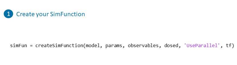
Create a SimFunction object using the createSimFunction method by choosing:

  1. which parameters it should take as inputs
  2. which targets will be dosed
  3. which model quantities it should return
  4. which sensitivities it should return if any

Have a look at the following example from the SimBiology documentation for an executable script to help you get started: Perform a Parameter Scan.