Results for
Hi guys could u guys please help me explain what is happening on this 3 graphs. I am an electrical student and just to be honest i am not a smart student but I'm willing to learn. Please do help me.Ive got my simulation i managed to generate perfect sin wave but i just couldn't explain on the graphs i simulated.
With the need for higher sampling frequencies, power electronics control engineers are moving some of their controller implementations to FPGAs or FPGA-based SoCs. Besides the use of wide-band gap semiconductors (GaN and SiC), what other reasons are driving the need for higher controller sampling frequencies? Let us know your thoughts.
If you have not seen this yet, in Release 2018b we added several examples to Simulink Control Design that show how to use this product to tune the gains of field-oriented controllers.
The first two examples make use of Closed-Loop PID Autotuner block . We show how to use this block to tune multiple loops in the motor control system, one loop at a time.
One of the examples shows tuning the controller gains for a PMSM:
Tune Field-Oriented Controllers Using Closed-Loop PID Autotuner Block
The other example shows how to tune four loops for an asynchronous machine (inductance motor):
Tune Field-Oriented Controllers for an Asynchronous Machine Using Closed-Loop PID Autotuner Block
This approach works well when you have initial gains that provide stable response, and you want to fine tune the controller to improve performance.
What do you do when you start with a new design and need to design your controller from scratch? That is what the third example is showing. Here we design all 3 loops (id, iq, speed) for a PMSM by running an AC sweep to compute a frequency response, then identifying a state-space model using System Identification Toolbox, and finally tuning all 3 loops simultaneously to provide desired performance.
Check it out here:
Tune Field-Oriented Controllers Using SYSTUNE
What do you think about these examples?
Share your opinion.
Arkadiy
On Wednesday, April 17, 12-1 PM EDT, Dr. Ing. Markus Rehberg, QSP Scientist at Sanofi in Frankfurt (Germany) will show how Sanofi and Rosa & Co created a QSP model for Rheumatoid Arthritis, using SimBiology, that transformed the way Sanofi uses and implements data in drug research and early development.
I invite you to register for the webinar, and afterward let me know what you think: https://register.gotowebinar.com/register/325575685872200717
What is it?
SimFunction allows you to perform multiple simulations in a single line of code by providing an interface to execute SimBiology® models like a regular MATLAB function.
Consider the following similarity: If you want to calculate the value of the sine function at multiple times defined in the variable t, you use the following syntax:
>> y = sin(t)
If mymodel represents a SimFunction, you can simulate your model with multiple parameter sets using the following syntax:
>> simulationData = mymodel(parameterValues, stopTime, dose)
What is it good for?
Multiple simulations
Because it allows you to perform multiple simulations in a single line of code by providing a matrix of parameter values or variants or a cell array of dosing tables, it is particularly suited for
- parameter and dose scans
- Monte Carlo simulations
- customized analyses that require multiple model simulations such as a customized optimization
Performance
SimFunctions are optimized for performance as they are automatically accelerated at the first function execution, which converts the model into compiled C code. Those simulations can be distributed to multiple cores or to a cluster and run in parallel if Parallel Computing Toolbox™ is available thanks to its built-in parallelization or within a parfor loop.
Simulation deployment
Since SimFunction objects cannot be changed once created, they can be shared with others without the risk of altering the model inadvertently.
Also, you can use SimFunctions to integrate a SimBiology model into a customized MATLAB App and compile it as standalone application to share with anyone without the need of a MATLAB license.
How does it work?
Create a SimFunction object using the createSimFunction method by choosing:
- which parameters it should take as inputs
- which targets will be dosed
- which model quantities it should return
- which sensitivities it should return if any
Have a look at the following example from the SimBiology documentation for an executable script to help you get started: Perform a Parameter Scan.
We are often asked to help with parameter estimation problems. This discussion aims to provide guidance for parameter estimation, as well as troubleshooting some of the more common failure modes. We welcome your thoughts and advice in the comments below.
Guidance and Best Practices:
1. Make sure your data is formatted correctly. Your data should have:
- a time column (defined as independent variable) that is monotonically increasing within every grouping variable,
- one or more concentration columns (dependent variable),
- one or more dose columns (with associated rate, if applicable) if you want your model to be perturbed by doses,
- a column with a grouping variable is optional.
Note: the dose column should only have entries at time points where a dose is administered. At time points where the dose is not administered, there should be no entry. When importing your data, MATLAB/SimBiology will replace empty cells with NaNs. Similarly, the concentration column should only have entries where measurements have been acquired and should be left empty otherwise.

If you import your data first in MATLAB, you can manipulate your data into the right format using datatype ' table ' and its methods such as sortrows , join , innerjoin , outerjoin , stack and unstack . You can then add the data to SimBiology by using the 'Import data from MATLAB workspace' functionality.
2. Visually inspect data and model response. Create a simulation task in the SimBiology desktop where you plot your data ( plot external data ), together with your model response. You can create sliders for the parameters you are trying to estimate (or use group simulation). You can then see whether, by varying these parameter values, you can bring the model response in line with your data, while at the same time giving you good initial estimates for those parameters. This plot can also indicate whether units might cause a discrepancy between your simulations and data, and/or whether doses administered to the model are configured correctly and result in a model response.
3. Determine sensitivity of your model response to model parameters. The previous section can be considered a manual sensitivity analysis. There is also a more systematic way of performing such an analysis: a global or local sensitivity analysis can be used to determine how sensitive your responses are to the parameters you are trying to estimate. If a model is not sensitive to a parameter, the parameter’s value may change significantly but this does not lead to a significant change in the model response. As a result, the value of the objective function is not sensitive to changes in that parameter value, hindering estimating the parameter’s value effectively.
4. Choose an optimization algorithm. SimBiology supports a range of optimization algorithms, depending on the toolboxes you have installed. As a default, we would recommend using lsqnonlin if you have access to the Optimization Toolbox. See troubleshooting below for more considerations choosing an appropriate optimization algorithm.
5. Map your data to your model components: Make sure the columns for your dependent variable(s) and dose(s) are mapped to the corresponding component(s) in your model.
6. Start small: bring the estimation task down to the smallest meaningful objective. If you want to estimate 10 parameters, try to start with estimating one or two instead. This will make troubleshooting easier. Once your estimation is set up properly with a few parameters, you can increase the number of parameters.
Troubleshooting
1. Are you trying to estimate a parameter that is governed by a rule? You can’t estimate parameters that are the subject of a rule (initial/repeated assignment, algebraic rule, rate rule), as the rule would supersede the value of the parameter you are trying to estimate. See this topic.
2. Is the optimization using the correct initial conditions and parameter values? Check whether - for the fit task - the parameter values and initial conditions that are used for the model, make sense. You can do this by passing the relevant dose(s) and variant(s) to the getequations function. In the SimBiology App, you can look at your equation view (When you have your model open, in the Model Tab, click Open -> Equations). Subsequently, - in the Model tab - click "Show Tasks" and select your fit task and inspect the initial conditions for your parameters and species. A typical example of this is when you do a dosing species but ka (the absorption rate) is set to zero. In that case, your dose will not transfer into the model and you will not see a model response.
3. Are your units consistent between your data and your model? You can use unit conversion to automatically achieve this.
4. Have you checked your solver tolerances? The absolute and relative tolerance of your solver determine how accurate your model simulation is. If a state in your model is on the order of 1e-9 but your tolerances only allow you to calculate this state with an accuracy down to 1e-8, your state will practically represent a random error around 1e-8. This is especially relevant if your data is on an order that is lower than your solver tolerances. In that case, your objective function will only pick up the solver error, rather than the true model response and will not be able to effectively estimate parameters. When you plot your data and model response together and by using a log-scale on the y-axis (right-click on your Live plot, select Properties, select Axes Properties, select Log scale under “Y-axis”) you can also see whether your ODE solver tolerances are sufficiently small to accurately compute model responses at the order of magnitude of your data. A give-away that this is not the case is when your model response appears to randomly vary as it bottoms-out around absolute solver tolerance.
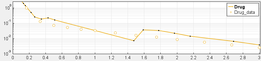
_ Tolerances are too low to simulate at the order of magnitude of the data. Absolute Tolerance: 0.001, Relative Tolerance: 0.01_
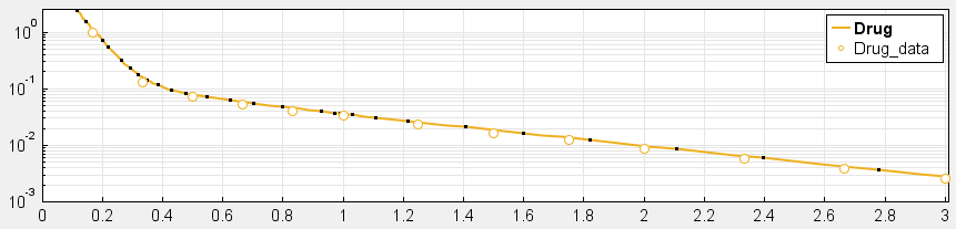
_ Sufficiently high tolerances. Absolute Tolerance: 1e-8, Relative Tolerance: 1e-5_
5. Have you checked the tolerances and stopping criteria of your optimization algorithm? The goal for your optimization should be that it terminates because it meets the imposed tolerances rather than because it exceeds the maximum number of iterations. Optimization algorithms terminate the estimation based on tolerances and stopping criteria. An example of a tolerance here is that you specify the precision with which you want to estimate a certain parameter, e.g. Cl with a precision down to 0.1 ml/hour. If these tolerances and stopping criteria are not set properly, your optimization could terminate early (leading to loss of precision in the estimation) or late (leading to unnecessarily long optimization compute times).
6. Have you considered structural and practical identifiability of your parameters? In your model, there might exist values for two (or more) parameters that result in a very similar model response. When estimating these parameters, the objective function will be very similar for these two parameters, resulting in the optimization algorithm not being able to find a unique set of parameter estimates. This effect is sometimes called aliasing and is a structural identifiability problem. An example would be if you have parallel enzymatic (Km, Vm) and linear clearance (Cl) routes. Practical identifiability occurs when there is not enough data available to sufficiently constrain the parameters you are estimating. An example is estimating the intercompartmental clearance (Q12), when you only have data on the central compartment of a two-compartment model. Another example would be that your data does not capture the process you are trying to estimate, e.g. you don’t have data on the absorption phase but are trying to estimate the absorption constant (Ka).
7. Have you considered trying another optimization algorithm? SimBiology supports a range of optimization algorithms, depending on the toolboxes you have installed. There is no single answer as to which algorithm you should use but some general guidelines can help in selecting the best algorithm.
- Non-linear regression: If your aim is to estimate parameters estimates for each group in your dataset (unpooled) or for all groups (pooled), you can use non-linear regression estimation methods. The optimization algorithms can be broken down into local and global optimization algorithms. You can use a local optimization algorithm when you have good initial estimates for the parameters you are trying to estimate. Each of the local optimization functions has a different default optimization algorithm: fminsearch (Nelder-Mead/downhill simplex search method), fmincon (interior-point), fminunc (quasi-newton), nlinfit (Levenberg-Marquardt), lsqcurvefit, lsqnonlin (both trust-region-reflective algorithm). As a default, we would recommend using lsqnonlin if you have access to the Optimization Toolbox. Note that all but the fminsearch algorithm are gradient based. If a gradient based algorithm fails to find suitable estimates, you can try fminsearch and see whether that improves the optimization. All local optimization algorithms can get “stuck” in a local minimum of the objective function and might therefore fail to reach the true minimum. Global optimization algorithms are developed to find the absolute minimum of the objective function. You can use global optimization algorithms when your fitting task results in different parameter estimates when repeated with different initial values (in other words, your optimization is getting stuck in local minima). You are more likely to encounter this as you increase the number of parameters you are estimating, as you increase the parameter space you are exploring (in other words, the bounds you are imposing on your estimates) and when you have poor initial estimates (in other words, your initial estimates are potentially very far from the estimates that correspond with the minimum of the objective function). A disadvantage of global optimization algorithms is that these algorithms are much more computationally expensive – they often take significantly more time to converge than the local optimization methods do. When using global optimization methods, we recommend using SimBiology’s built-in scattersearch algorithm, combined with lsqnonlin as a local solver. If you have access to the Global Optimization Toolbox, you can try the functions ga (genetic algorithm), patternsearch and particleswarm. Note that some of the global optimization algorithms, including scattersearch, lend themselves well to be accelerated using parallel or distributed computing.
- Estimate category-specific parameters: If you want to estimate category-specific parameters for multiple subjects, e.g. you have 10 male and 10 female subjects in your dataset and you want to estimate a separate clearance value for each gender while all other parameters will be gender-independent, you can also use non-linear regression. Please refer to this example in the documentation.
- Non-linear mixed effects: If your data represents a population of individuals where you think there could be significant inter-individual variability you can use mixed effects modeling to estimate the fixed and random effects present in your population, while also understanding covariance between different parameters you are trying to estimate. When performing mixed effects estimation, it is advisable to perform fixed effects estimation in order to obtain reasonable initial estimates for the mixed effects estimation. SimBiology supports two estimation functions: nlmefit (LME, RELME, FO or FOCE algorithms), and nlmefitsa (Stochastic Approximation Expectation-Maximization). Sometimes, these solvers might seem to struggle to converge. In that case, it is worthwhile determining whether your (objective) function tolerance is set too low and increasing the tolerance somewhat.
8. Does your optimization get stuck? Sometimes, the optimization algorithm can get stuck at a certain iteration. For a particular iteration, the parameter values that model is simulated with as part of the optimization process, can cause the model to be in a state where the ODE solver needs to take very small time-steps to achieve the tolerances (e.g. very rapid changes of model responses). Solutions can include: changing your initial estimates, imposing lower and upper bounds on the parameters you are trying to estimate, selecting to a different solver, easing solver tolerances (only where possible, see also “Visually inspect data and model response”).
9. Are you using the proportional error model? The objective function for the proportional error model contains a term where your response data is part of the denominator. As response variables get close to zero or are exactly zero, this effectively means the objective function contains one or more terms that divide by zero, causing errors or at least very slow iterations of your optimization algorithm. You can try to change the error model to constant or combined to circumvent this problem. Alternatively, you can define separate error models for each response: proportional for those responses that don’t have measurements that contain values close to zero and a constant error model for those responses that do.
Dear all,
I am new to SimBiology. I am doing my research in Molecular Communication. Recently I have found out that SimBiology can be used for simulating the Bit Error Rate performance of molecular Communication systems. Please help me to find good reference materials/examples for using SimBiology as a simulation tool for Molecular Communications.
Thank you.
Tomorrow (Wednesday, January 23) during Rosa's Impact of Modeling & Simulation in Drug Development webinar series, Chi-Chung Li, a Senior Scientist at Genentech, will present a case study where SimBiology was used to create a QSP model that enhanced decision making in a Phase I trial.
Sign up now and have the ability to ask questions at the end of the webinar, or access the archived version later: https://www.rosaandco.com/webinars/2019/phase-i-clinical-decision-making-qsp-case-study

AI and ACoP, hype or real?
Iraj Hosseini, Ph.D., of Genentech will present a webinar on gPKPDSim , a MATLAB app that facilitates non-modelers to explore and simulate PKPD models built in SimBiology.
While model development typically requires mathematical modeling expertise, model exploration and simulation could be performed by non-modeler scientists to support experimental studies. Dr. Hosseini and his colleagues collaborate with MathWorks' consulting services to develop an App to enable easy use of any model constructed in SimBiology to execute common PKPD analyses.
Webinar will be hosted by Rosa & Co. on Wednesday October 24. To register, go to: https://register.gotowebinar.com/register/7922912955745684993?mw
This project presents a SimBiology implementation of Mager and Jusko’s generic Target-Mediated Drug Disposition model (TMDD) as described in "General pharmacokinetic model for drugs exhibiting target-mediated drug disposition". Target-mediated drug disposition is a common source of nonlinearity in PK profiles for biotherapeutics. Nonlinearities are introduced because drug-target bindings saturate at therapeutic dosing levels.
Drug in the Plasma reversibly binds with the unbound Target to form drug-target Complex. kon and koff are the association and dissociation rate constants, and clearance of free Drug and Complex from the Plasma is described by first-order processes with rate constants, kel and km, respectively. Free target turnover is described by a zero-order synthesis rate, ksyn, and a first order elimination (rate constant, kdeg). The model also includes an optional Tissue compartment to account for non-specific tissue binding or distribution.

References [1] Mager DE and Jusko WJ (2001) General pharmacokinetic model for drugs exhibiting target-mediated drug disposition. J Pharmacokinetics and Pharmacodynamics 28: 507–532.
This project presents SimBiology model implementation of the systemic Renin-Angiotensin-System that was first developed by Lo et al. and used to investigate the effects of different RAS-modulating therapies. The RAS pathway is crucial for blood pressure and kidney function control as well as a range of other organism-wide functions. The model describes the enzymatic conversion of the precursor protein Angiotensinogen to Angiotensin I and its downstream products Angiotensin 1-7, Angiotensin II and Angiotensin IV. Key pathway effects are triggered by the association of Angiotensin II with the AT1-Receptor. A positive feedback loop connects the Angiotensin II–AT1-Receptor complex with the Angiotensinogen conversion (not shown in the diagram). Enzymatic reactions are modeled as pseudo-unimolecular using enzymatic activities as reaction rates. Degradation reactions are described using protein half-life times. Drug pharmacodynamics are included in the model using the term (1-DrugEffect), where DrugEffect follows a sigmoidal dependence on the Drug concentration, to modify the target enzyme activity.
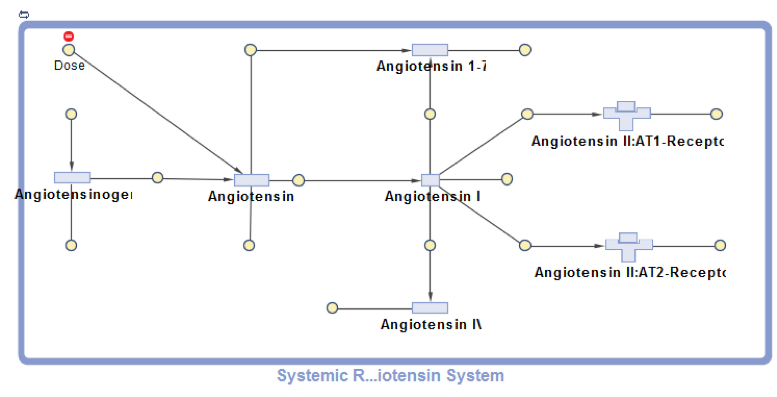
References [1] Lo, A., Beh, J., Leon, H. D., Hallow, M. K., Ramakrishna, R., Rodrigo, M., & Sarkar, A. (2011). Using a Systems Biology Approach to Explore Hypotheses Underlying Clinical Diversity of the Renin Angiotensin System and the Response to Antihypertensive Therapies. Clinical Trial Simulations, 1, 457–482.
This project presents a SimBiology implementation of a physiologically-based pharmacokinetic (PBPK) model for trichloroethylene (TCE) and its metabolites. It is based on the article, “A human physiologically based pharmacokinetic model for trichloroethylene and its metabolites, trichloroacetic acid and free trichloroethanol” by Fisher et al. [1].
The human PBPK model for TCE and its metabolites presented here was developed by Fisher et al. [1] in order to assess human health risks associated with low level exposure to TCE. TCE is a commonly used solvent in the automotive and metal industries for vapor degreasing of metal parts. Exposure to TCE has been associated with toxic responses such as cancer formation and brain disorders in rodents and in humans [1]. In this PBPK model, TCE enters the systemic circulation through inhalation. Its disposition is described by a six-compartment model representing the liver, lung, kidney, fat, and slowly perfused and rapidly perfused tissues. In the liver, TCE is metabolized to trichloroacetic acid (TCA) and free trichloroethanol (TCOH-f) via P450-mediated metabolism where a fraction of TCOH-f is converted to TCA. For simplicity, a four-compartment submodel was used to describe the disposition of metabolites, TCA and TCOH-f, in the lung, liver, kidney, and body (muscle). Both metabolites are described to be excreted in the urine. TCOH-f is glucuronidated in the liver, forming glucuronide-bound TCOH (TCOH-b), and excreted in the urine via a saturable process whereas TCA is excreted by a first-order process by the kidney.

Reference: Fisher, J. W., Mahle, D., & Abbas, R. (1998). A human physiologically based pharmacokinetic model for trichloroethylene and its metabolites, trichloroacetic acid and free trichloroethanol. Toxicology and applied pharmacology, 152(2), 339-359.
Hi there! This is kind of an unusual question, but here it goes. I am a big time Matlab enthusiast and I met some of your representatives at Formula Student Germany back in August. There was a booth were your product was showcased but most importantly there was Matlab merchandise such as stickers, rub-on-tattoos and pens with the mathworks logo being handed out. This merchandise is increadibly popular with me and my nerdy friends. But sadly I didnt bring much with me from the event. Is it possible to get ahold some of it? Is it for sale? Are you willing to sponsor some geeky engineering students?