Main Content

Results for


An option for 10th degree polynomials but no weighted linear least squares. Seriously? Jesse
Twitch built an entire business around letting you watch over someone's shoulder while they play video games. I feel like we should be able to make at least a few videos where we get to watch over someone's shoulder while they solve Cody problems. I would pay good money for a front-row seat to watch some of my favorite solvers at work. Like, I want to know, did Alfonso Nieto-Castonon just sit down and bang out some of those answers, or did he have to think about it for a while? What was he thinking about while he solved it? What resources was he drawing on? There's nothing like watching a master craftsman at work.
I can imagine a whole category of Cody videos called "How I Solved It". I tried making one of these myself a while back, but as far as I could tell, nobody else made one.
Here's the direct link to the video: https://www.youtube.com/watch?v=hoSmO1XklAQ
I hereby challenge you to make a "How I Solved It" video and post it here. If you make one, I'll make another one.
The Ans Hack is a dubious way to shave a few points off your solution score. Instead of a standard answer like this
function y = times_two(x)
y = 2*x;
end
you would do this
function ans = times_two(x)
2*x;
end
The ans variable is automatically created when there is no left-hand side to an evaluated expression. But it makes for an ugly function. I don't think anyone actually defends it as a good practice. The question I would ask is: is it so offensive that it should be specifically disallowed by the rules? Or is it just one of many little hacks that you see in Cody, inelegant but tolerable in the context of the surrounding game?
Incidentally, I wrote about the Ans Hack long ago on the Community Blog. Dealing with user-unfriendly code is also one of the reasons we created the Head-to-Head voting feature. Some techniques are good for your score, and some are good for your code readability. You get to decide with you care about.
While searching the internet for some books on ordinary differential equations, I came across a link that I believe is very useful for all math students and not only. If you are interested in ODEs, it's worth taking the time to study it.
A First Look at Ordinary Differential Equations by Timothy S. Judson is an excellent resource for anyone looking to understand ODEs better. Here's a brief overview of the main topics covered:
  1. Introduction to ODEs: Basic concepts, definitions, and initial differential equations.
  2. Methods of Solution:
  • Separable equations
  • First-order linear equations
  • Exact equations
  • Transcendental functions
  1. Applications of ODEs: Practical examples and applications in various scientific fields.
  2. Systems of ODEs: Analysis and solutions of systems of differential equations.
  3. Series and Numerical Methods: Use of series and numerical methods for solving ODEs.
This book provides a clear and comprehensive introduction to ODEs, making it suitable for students and new researchers in mathematics. If you're interested, you can explore the book in more detail here: A First Look at Ordinary Differential Equations.
goc3
goc3
Last activity on 7 Jun 2024

There are a host of problems on Cody that require manipulation of the digits of a number. Examples include summing the digits of a number, separating the number into its powers, and adding very large numbers together.
If you haven't come across this trick yet, you might want to write it down (or save it electronically):
digits = num2str(4207) - '0'
That code results in the following:
digits =
4 2 0 7
Now, summing the digits of the number is easy:
sum(digits)
ans =
13
Hello and a warm welcome to everyone! We're excited to have you in the Cody Discussion Channel. To ensure the best possible experience for everyone, it's important to understand the types of content that are most suitable for this channel.
Content that belongs in the Cody Discussion Channel:
  • Tips & tricks: Discuss strategies for solving Cody problems that you've found effective.
  • Ideas or suggestions for improvement: Have thoughts on how to make Cody better? We'd love to hear them.
  • Issues: Encountering difficulties or bugs with Cody? Let us know so we can address them.
  • Requests for guidance: Stuck on a Cody problem? Ask for advice or hints, but make sure to show your efforts in attempting to solve the problem first.
  • General discussions: Anything else related to Cody that doesn't fit into the above categories.
Content that does not belong in the Cody Discussion Channel:
  • Comments on specific Cody problems: Examples include unclear problem descriptions or incorrect testing suites.
  • Comments on specific Cody solutions: For example, you find a solution creative or helpful.
Please direct such comments to the Comments section on the problem or solution page itself.
We hope the Cody discussion channel becomes a vibrant space for sharing expertise, learning new skills, and connecting with others.
๐Ÿ“š New Book Announcement: "Image Processing Recipes in MATLAB" ๐Ÿ“š
I am delighted to share the release of my latest book, "Image Processing Recipes in MATLAB," co-authored by my dear friend and colleague Gustavo Benvenutti Borba.
This 'cookbook' contains 30 practical recipes for image processing, ranging from foundational techniques to recently published algorithms. It serves as a concise and readable reference for quickly and efficiently deploying image processing pipelines in MATLAB.
Gustavo and I are immensely grateful to the MathWorks Book Program for their support. We also want to thank Randi Slack and her fantastic team at CRC Press for their patience, expertise, and professionalism throughout the process.
___________
A high school student called for help with this physics problem:
  • Car A moves with constant velocity v.
  • Car B starts to move when Car A passes through the point P.
  • Car B undergoes...
  • uniform acc. motion from P to Q.
  • uniform velocity motion from Q to R.
  • uniform acc. motion from R to S.
  • Car A and B pass through the point R simultaneously.
  • Car A and B arrive at the point S simultaneously.
Q1. When car A passes the point Q, which is moving faster?
Q2. Solve the time duration for car B to move from P to Q using L and v.
Q3. Magnitude of acc. of car B from P to Q, and from R to S: which is bigger?
Well, it can be solved with a series of tedious equations. But... how about this?
Code below:
%% get images and prepare stuffs
figure(WindowStyle="docked"),
ax1 = subplot(2,1,1);
hold on, box on
ax1.XTick = [];
ax1.YTick = [];
A = plot(0, 1, 'ro', MarkerSize=10, MarkerFaceColor='r');
B = plot(0, 0, 'bo', MarkerSize=10, MarkerFaceColor='b');
[carA, ~, alphaA] = imread('https://cdn.pixabay.com/photo/2013/07/12/11/58/car-145008_960_720.png');
[carB, ~, alphaB] = imread('https://cdn.pixabay.com/photo/2014/04/03/10/54/car-311712_960_720.png');
carA = imrotate(imresize(carA, 0.1), -90);
carB = imrotate(imresize(carB, 0.1), 180);
alphaA = imrotate(imresize(alphaA, 0.1), -90);
alphaB = imrotate(imresize(alphaB, 0.1), 180);
carA = imagesc(carA, AlphaData=alphaA, XData=[-0.1, 0.1], YData=[0.9, 1.1]);
carB = imagesc(carB, AlphaData=alphaB, XData=[-0.1, 0.1], YData=[-0.1, 0.1]);
txtA = text(0, 0.85, 'A', FontSize=12);
txtB = text(0, 0.17, 'B', FontSize=12);
yline(1, 'r--')
yline(0, 'b--')
xline(1, 'k--')
xline(2, 'k--')
text(1, -0.2, 'Q', FontSize=20, HorizontalAlignment='center')
text(2, -0.2, 'R', FontSize=20, HorizontalAlignment='center')
% legend('A', 'B') % this make the animation slow. why?
xlim([0, 3])
ylim([-.3, 1.3])
%% axes2: plots velocity graph
ax2 = subplot(2,1,2);
box on, hold on
xlabel('t'), ylabel('v')
vA = plot(0, 1, 'r.-');
vB = plot(0, 0, 'b.-');
xline(1, 'k--')
xline(2, 'k--')
xlim([0, 3])
ylim([-.3, 1.8])
p1 = patch([0, 0, 0, 0], [0, 1, 1, 0], [248, 209, 188]/255, ...
EdgeColor = 'none', ...
FaceAlpha = 0.3);
%% solution
v = 1; % car A moves with constant speed.
L = 1; % distances of P-Q, Q-R, R-S
% acc. of car B for three intervals
a(1) = 9*v^2/8/L;
a(2) = 0;
a(3) = -1;
t_BatQ = sqrt(2*L/a(1)); % time when car B arrives at Q
v_B2 = a(1) * t_BatQ; % speed of car B between Q-R
%% patches for velocity graph
p2 = patch([t_BatQ, t_BatQ, t_BatQ, t_BatQ], [1, 1, v_B2, v_B2], ...
[248, 209, 188]/255, ...
EdgeColor = 'none', ...
FaceAlpha = 0.3);
p3 = patch([2, 2, 2, 2], [1, v_B2, v_B2, 1], [194, 234, 179]/255, ...
EdgeColor = 'none', ...
FaceAlpha = 0.3);
%% animation
tt = linspace(0, 3, 2000);
for t = tt
A.XData = v * t;
vA.XData = [vA.XData, t];
vA.YData = [vA.YData, 1];
if t < t_BatQ
B.XData = 1/2 * a(1) * t^2;
vB.XData = [vB.XData, t];
vB.YData = [vB.YData, a(1) * t];
p1.XData = [0, t, t, 0];
p1.YData = [0, vB.YData(end), 1, 1];
elseif t >= t_BatQ && t < 2
B.XData = L + (t - t_BatQ) * v_B2;
vB.XData = [vB.XData, t];
vB.YData = [vB.YData, v_B2];
p2.XData = [t_BatQ, t, t, t_BatQ];
p2.YData = [1, 1, vB.YData(end), vB.YData(end)];
else
B.XData = 2*L + v_B2 * (t - 2) + 1/2 * a(3) * (t-2)^2;
vB.XData = [vB.XData, t];
vB.YData = [vB.YData, v_B2 + a(3) * (t - 2)];
p3.XData = [2, t, t, 2];
p3.YData = [1, 1, vB.YData(end), v_B2];
end
txtA.Position(1) = A.XData(end);
txtB.Position(1) = B.XData(end);
carA.XData = A.XData(end) + [-.1, .1];
carB.XData = B.XData(end) + [-.1, .1];
drawnow
end
Chen Lin
Chen Lin
Last activity on 3 Jul 2024

Northern lights captured from this weekend at MathWorks campus โœจ
Did you get a chance to see lights and take some photos?
Updating some of my educational Livescripts to 2024a, really love the new "define a function anywhere" feature, and have a "new" idea for improving Livescripts -- support "hidden" code blocks similar to the Jupyter Notebooks functionality.
For example, I often create "complicated" plots with a bunch of ancillary items and I don't want this code exposed to the reader by default, as it might confuse the reader. For example, consider a Livescript that might read like this:
-----
Noting the similar structure of these two mappings, let's now write a function that simply maps from some domain to some other domain using change of variable.
function x = ChangeOfVariable( x, from_domain, to_domain )
x = x - from_domain(1);
x = x * ( ( to_domain(2) - to_domain(1) ) / ( from_domain(2) - from_domain(1) ) );
x = x + to_domain(1);
end
Let's see this function in action
% HIDE CELL
clear
close all
from_domain = [-1, 1];
to_domain = [2, 7];
from_values = [-1, -0.5, 0, 0.5, 1];
to_values = ChangeOfVariable( from_values, from_domain, to_domain )
to_values = 1ร—5
2.0000 3.2500 4.5000 5.7500 7.0000
We can plot the values of from_values and to_values, showing how they're connected to each other:
% HIDE CELL
figure
hold on
for n = 1 : 5
plot( [from_values(n) to_values(n)], [1 0], Color="k", LineWidth=1 )
end
ax = gca;
ax.YTick = [];
ax.XLim = [ min( [from_domain, to_domain] ) - 1, max( [from_domain, to_domain] ) + 1 ];
ax.YLim = [-0.5, 1.5];
ax.XGrid = "on";
scatter( from_values, ones( 5, 1 ), Marker="s", MarkerFaceColor="flat", MarkerEdgeColor="k", SizeData=120, LineWidth=1, SeriesIndex=1 )
text( mean( from_domain ), 1.25, "$\xi$", Interpreter="latex", HorizontalAlignment="center", VerticalAlignment="middle" )
scatter( to_values, zeros( 5, 1 ), Marker="o", MarkerFaceColor="flat", MarkerEdgeColor="k", SizeData=120, LineWidth=1, SeriesIndex=2 )
text( mean( to_domain ), -0.25, "$x$", Interpreter="latex", HorizontalAlignment="center", VerticalAlignment="middle" )
scaled_arrow( ax, [mean( [from_domain(1), to_domain(1) ] ) - 1, 0.5], ( 1 - 0 ) / ( from_domain(1) - to_domain(1) ), 1 )
scaled_arrow( ax, [mean( [from_domain(end), to_domain(end)] ) + 1, 0.5], ( 1 - 0 ) / ( from_domain(end) - to_domain(end) ), -1 )
text( mean( [from_domain(1), to_domain(1) ] ) - 1.5, 0.5, "$x(\xi)$", Interpreter="latex", HorizontalAlignment="center", VerticalAlignment="middle" )
text( mean( [from_domain(end), to_domain(end)] ) + 1.5, 0.5, "$\xi(x)$", Interpreter="latex", HorizontalAlignment="center", VerticalAlignment="middle" )
-----
Where scaled_arrow is some utility function I've defined elsewhere... See how a majority of the code is simply "drivel" to create the plot, clear and close? I'd like to be able to hide those cells so that it would look more like this:
-----
Noting the similar structure of these two mappings, let's now write a function that simply maps from some domain to some other domain using change of variable.
function x = ChangeOfVariable( x, from_domain, to_domain )
x = x - from_domain(1);
x = x * ( ( to_domain(2) - to_domain(1) ) / ( from_domain(2) - from_domain(1) ) );
x = x + to_domain(1);
end
Let's see this function in action
โ–ถ Show code cell
from_domain = [-1, 1];
to_domain = [2, 7];
from_values = [-1, -0.5, 0, 0.5, 1];
to_values = ChangeOfVariable( from_values, from_domain, to_domain )
to_values = 1ร—5
2.0000 3.2500 4.5000 5.7500 7.0000
We can plot the values of from_values and to_values, showing how they're connected to each other:
โ–ถ Show code cell
-----
Thoughts?
I recently had issues with code folding seeming to disappear and it turns out that I had unknowingly disabled the "show code folding margin" option by accident. Despite using MATLAB for several years, I had no idea this was an option, especially since there seemed to be no references to it in the code folding part of the "Preferences" menu.
It would be great if in the future, there was a warning that told you about this when you try enable/disable folding in the Preferences.
I am using 2023b by the way.
In the MATLAB editor, when clicking on a variable name, all the other instances of the variable name will be highlighted.
But this does not work for structure fields, which is a pity. Such feature would be quite often useful for me.
I show an illustration below, and compare it with Visual Studio Code that does it. ;-)
I am using MATLAB R2023a, sorry if it has been added to newer versions, but I didn't see it in the release notes.

Hello MathWorks Community,

I am excited to announce that I am currently working on a book project centered around Matrix Algebra, specifically designed for MATLAB users. This book aims to cater to undergraduate students in engineering, where Matrix Algebra serves as a foundational element.

Matrix Algebra is not only pivotal in understanding complex engineering concepts but also in applying these principles effectively in various technological solutions. MATLAB, renowned for its powerful computational capabilities, is an excellent tool to explore and implement these concepts, making it a perfect companion for this book.

As I embark on this journey to create a resource that bridges theoretical matrix algebra with practical MATLAB applications, I am looking for one or two knowledgeable individuals who have a firm grasp of both subjects. If you have experience in teaching or applying matrix algebra in engineering contexts and are familiar with MATLAB, your contribution could be invaluable.

Collaborators will help in shaping the content to ensure it is educational, engaging, and technically robust, making complex concepts accessible and applicable for students.

If you are interested in contributing to this project or know someone who might be, please reach out to discuss how we can work together to make this book a valuable resource for engineering students.

Thank you and looking forward to your participation!

Chen Lin
Chen Lin
Last activity on 12 Apr 2024

What's the weather like in your place?
David
David
Last activity on 2 Apr 2024

I feel like no one at UC San Diego knows this page, let alone this server, is still live. For the younger generation, this is what the whole internet used to look like :)
In short: support varying color in at least the plot, plot3, fplot, and fplot3 functions.
This has been a thing that's come up quite a few times, and includes questions/requests by users, workarounds by the community, and workarounds presented by MathWorks -- examples of each below. It's a feature that exists in Python's Matplotlib library and Sympy. Anyways, given that there are myriads of workarounds, it appears to be one of the most common requests for Matlab plots (Matlab's plotting is, IMO, one of the best features of the product), the request precedes the 21st century, and competitive tools provide the functionality, it would seem to me that this might be the next great feature for Matlab plotting.
I'm curious to get the rest of the community's thoughts... what's everyone else think about this?
---
User questions/requests
User-provided workarounds
MathWorks-provided workarounds
I would like to propose the creation of MATLAB EduHub, a dedicated channel within the MathWorks community where educators, students, and professionals can share and access a wealth of educational material that utilizes MATLAB. This platform would act as a central repository for articles, teaching notes, and interactive learning modules that integrate MATLAB into the teaching and learning of various scientific fields.
Key Features:
1. Resource Sharing: Users will be able to upload and share their own educational materials, such as articles, tutorials, code snippets, and datasets.
2. Categorization and Search: Materials can be categorized for easy searching by subject area, difficulty level, and MATLAB version..
3. Community Engagement: Features for comments, ratings, and discussions to encourage community interaction.
4. Support for Educators: Special sections for educators to share teaching materials and track engagement.
Benefits:
- Enhanced Educational Experience: The platform will enrich the learning experience through access to quality materials.
- Collaboration and Networking: It will promote collaboration and networking within the MATLAB community.
- Accessibility of Resources: It will make educational materials available to a wider audience.
By establishing MATLAB EduHub, I propose a space where knowledge and experience can be freely shared, enhancing the educational process and the MATLAB community as a whole.
Several of the colormaps are great for a 256 color surface plot, but aren't well optimized for extracting m colors for plotting several independent lines. The issue is that many colormaps have start/end colors that are too similar or are suboptimal colors for lines. There are certainly many workarounds for this, but it would be a great quality of life to adjust that directly when calling this.
Example:
x = linspace(0,2*pi,101)';
y = [1:6].*cos(x);
figure; plot(x,y,'LineWidth',2); grid on; axis tight;
And now if I wanted to color these lines, I could use something like turbo(6) or gray(6) and then apply it using colororder.
colororder(turbo(6))
But my issue is that the ends of the colormap are too similar. For other colormaps, you may get lines that are too light to be visible against the white background. There are plenty of workarounds, with my preference being to create extra colors and truncate that before using colororder.
cmap = turbo(8); cmap = cmap(2:end-1,:); % Truncate the end colors
figure; plot(x,y,'LineWidth',2); grid on; axis tight;
colororder(cmap)
I think it would be really awesome to add some name-argument input pair to these colormaps that can specify the range you want so this could even be done inside the colororder calling if desired. An example of my proposed solution would look something like this:
cmap = turbo(6,'Range',[0.1 0.8]); % Proposed idea to add functionality
Where in this scenario, the resulting colormap would be 6 equally spaced colors that range from 10% to 80% of the total color range. This would be especially nice because you could more quickly modify the range of colors, or you could set the limits regardless of whether you need to plot 3, 6, or 20 lines.
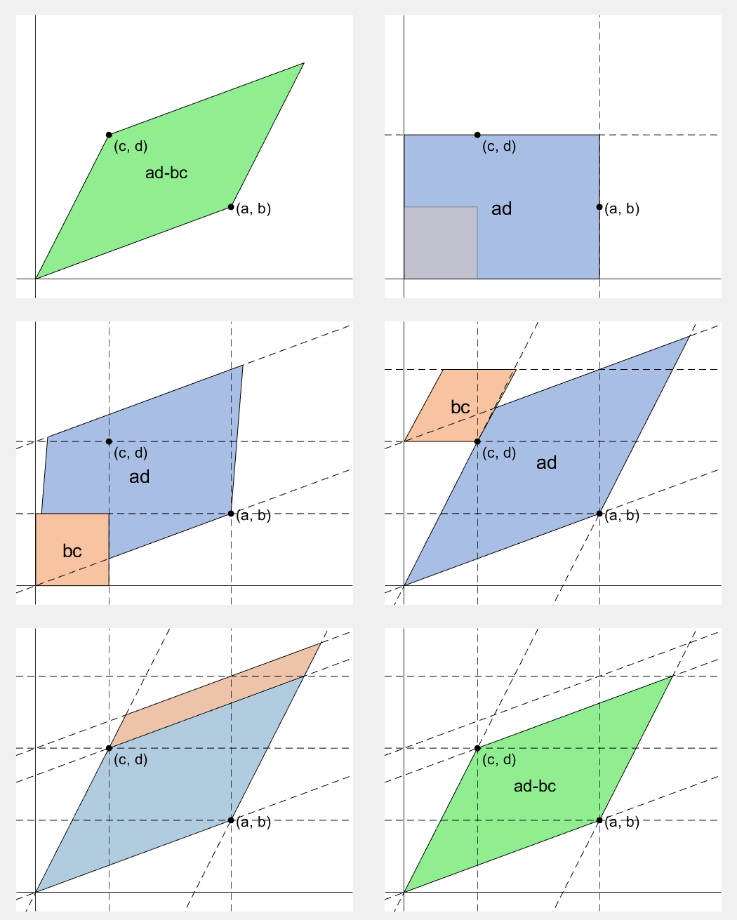
2 x 2 ํ–‰๋ ฌ์˜ ํ–‰๋ ฌ์‹์€
  • ํ–‰๋ ฌ์˜ ๋‘ row ๋ฒกํ„ฐ๋กœ ์ •์˜๋˜๋Š” ํ‰ํ–‰์‚ฌ๋ณ€ํ˜•์˜ ๋ฉด์ ์ž…๋‹ˆ๋‹ค.
  • ๋ฌผ๋ก  ๋‘ column ๋ฒกํ„ฐ๋กœ ์ •์˜๋˜๋Š” ํ‰ํ–‰์‚ฌ๋ณ€ํ˜•์˜ ๋ฉด์ ์ด๊ธฐ๋„ ํ•ฉ๋‹ˆ๋‹ค.
  • ์ข€ ๋” ์ •ํ™•ํžˆ๋Š” signed area์ž…๋‹ˆ๋‹ค. ๋ฉด์ ์ด ์Œ์ˆ˜๊ฐ€ ๋  ์ˆ˜๋„ ์žˆ๋‹ค๋Š” ๋œป์ด์ฃ .
  • ํ–‰๋ ฌ์˜ ๋‘ ํ–‰(๋˜๋Š” ๋‘ ์—ด)์„ ๋งž๋ฐ”๊พธ๋ฉด ํ–‰๋ ฌ์‹์˜ ๋ถ€ํ˜ธ๋„ ๋ฐ”๋€Œ๊ณ  ๋ฉด์ ์˜ ๋ถ€ํ˜ธ๋„ ๋ฐ”๋€Œ์–ด์•ผํ•ฉ๋‹ˆ๋‹ค.
์ผ๋ฐ˜์ ์œผ๋กœ n x n ํ–‰๋ ฌ์˜ ํ–‰๋ ฌ์‹์€
  • ๊ฐ row ๋ฒกํ„ฐ(๋˜๋Š” ๊ฐ column ๋ฒกํ„ฐ)๋กœ ์ •์˜๋˜๋Š” N์ฐจ์› ๊ณต๊ฐ„์˜ ํ‰ํ–‰๋ฉด์ฒด(?)์˜ signed area์ž…๋‹ˆ๋‹ค.
  • ์ œ๋Œ€๋กœ ์ดํ•ดํ•˜๋ ค๋ฉด ๋Œ€์ˆ˜ํ•™์˜ ๊ฐœ๋…์„ ๋งŽ์ด ๊ฐ€์ง€๊ณ  ์™€์•ผ ํ•˜๋Š”๋ฐ ์ž์„ธํ•œ ์„ค๋ช…์€ ์ƒ๋žตํ•ฉ๋‹ˆ๋‹ค.(=์ €๋„ ๋ชจ๋ฅธ๋‹ค๋Š” ๋œป)
  • ๋” ์ž์„ธํžˆ ์•Œ๊ณ  ์‹ถ์œผ์‹œ๋ฉด ์ˆ˜ํ•™ํ•˜๋Š” ๋งŒํ™”์˜ '๋„“์ด ์ด์•ผ๊ธฐ' ํŽธ์„ ์ถ”์ฒœํ•ฉ๋‹ˆ๋‹ค.
  • ์ˆ˜ํ•™์ ์ธ ์ •์˜๋ฅผ ์•Œ๊ณ  ์‹ถ์œผ์‹œ๋ฉด ์œ„ํ‚คํ”ผ๋””์•„๋ฅผ ๋ณด์‹œ๋ฉด ๋ฉ๋‹ˆ๋‹ค.
  • ์ด๋ ‡๊ฒŒ ์ƒ๊ฒผ์Šต๋‹ˆ๋‹ค. ์ข€ ๋ฌด์„ญ์Šต๋‹ˆ๋‹ค.
์•„๋ž˜ ์ฝ”๋“œ๋Š”...
  • 2 x 2 ํ–‰๋ ฌ์— ๋Œ€ํ•ด์„œ ์ด๊ฒƒ์„ ์ˆ˜์‹ ์—†์ด ๊ทธ๋ฆผ๋งŒ์œผ๋กœ ์ฆ๋ช…ํ•˜๋Š” ๊ณผ์ •์ž…๋‹ˆ๋‹ค.
  • gif ์ƒ์„ฑ์—๋Š” ScreenToGif๋ฅผ ์‚ฌ์šฉํ–ˆ์Šต๋‹ˆ๋‹ค. (gif ๋งŒ๋“ค๊ธฐ์—” ์ด๊ฒŒ ํ‚น์™•์งฑ์ธ๋“ฏ)
Determinant of 2 x 2 matrix is...
  • An area of a parallelogram defined by two row vectors.
  • Of course, same one defined by two column vectors.
  • Precisely, a signed area, which means area can be negative.
  • If two rows (or columns) are swapped, both the sign of determinant and area change.
More generally, determinant of n x n matrix is...
  • Signed area of parallelepiped defined by rows (or columns) of the matrix in n-dim space.
  • For a full understanding, a lot of concepts from abstract algebra should be brought, which I will not write here. (Cuz I don't know them.)
  • For a mathematical definition of determinant, visit wikipedia.
  • A little scary, isn't it?
The code below is...
  • A process to prove the equality of the determinant of 2 x 2 matrix and the area of parallelogram.
  • ScreenToGif is used to generate gif animation (which is, to me, the easiest way to make gif).
% ๋‘ ์  (a, b), (c, d)์˜ ์ขŒํ‘œ
a = 4;
b = 1;
c = 1;
d = 3;
% patch ์ƒ‰ pre-define
lightgreen = [144, 238, 144]/255;
lightblue = [169, 190, 228]/255;
lightorange = [247, 195, 160]/255;
% animation params.
anim_Nsteps = 30;
% create window
figure('WindowStyle','docked')
ax = axes;
ax.XAxisLocation = 'origin';
ax.YAxisLocation = 'origin';
ax.XTick = [];
ax.YTick = [];
hold on
ax.XLim = [-.4, a+c+1];
ax.YLim = [-.4, b+d+1];
% create ad-bc patch
area = patch([0, a, a+c, c], [0, b, b+d, d], lightgreen);
p_ab = plot(a, b, 'ko', 'MarkerFaceColor', 'k');
p_cd = plot(c, d, 'ko', 'MarkerFaceColor', 'k');
p_ab.UserData = text(a+0.1, b, '(a, b)', 'FontSize',16);
p_cd.UserData = text(c+0.1, d-0.2, '(c, d)', 'FontSize',16);
area.UserData = text((a+c)/2-0.5, (b+d)/2, 'ad-bc', 'FontSize', 18);
pause
%% Is this really ad-bc?
area.UserData.String = 'ad-bc...?';
pause
%% fade out ad-bc
fadeinout(area, 0)
area.UserData.Visible = 'off';
pause
%% fade in ad block
rect_ad = patch([0, a, a, 0], [0, 0, d, d], lightblue, 'EdgeAlpha', 0, 'FaceAlpha', 0);
uistack(rect_ad, 'bottom');
fadeinout(rect_ad, 1, t_pause=0.003)
draw_gridline(rect_ad, ["23", "34"])
rect_ad.UserData = text(mean(rect_ad.XData), mean(rect_ad.YData), 'ad', 'FontSize', 20, 'HorizontalAlignment', 'center');
pause
%% fade-in bc block
rect_bc = patch([0, c, c, 0], [0, 0, b, b], lightorange, 'EdgeAlpha', 0, 'FaceAlpha', 0);
fadeinout(rect_bc, 1, t_pause=0.0035)
draw_gridline(rect_bc, ["23", "34"])
rect_bc.UserData = text(b/2, c/2, 'bc', 'FontSize', 20, 'HorizontalAlignment', 'center');
pause
%% slide ad block
patch_slide(rect_ad, ...
[0, 0, 0, 0], [0, b, b, 0], t_pause=0.004)
draw_gridline(rect_ad, ["12", "34"])
pause
%% slide ad block
patch_slide(rect_ad, ...
[0, 0, d/(d/c-b/a), d/(d/c-b/a)],...
[0, 0, b/a*d/(d/c-b/a), b/a*d/(d/c-b/a)], t_pause=0.004)
draw_gridline(rect_ad, ["14", "23"])
pause
%% slide bc block
uistack(p_cd, 'top')
patch_slide(rect_bc, ...
[0, 0, 0, 0], [d, d, d, d], t_pause=0.004)
draw_gridline(rect_bc, "34")
pause
%% slide bc block
patch_slide(rect_bc, ...
[0, 0, a, a], [0, 0, 0, 0], t_pause=0.004)
draw_gridline(rect_bc, "23")
pause
%% slide bc block
patch_slide(rect_bc, ...
[d/(d/c-b/a), 0, 0, d/(d/c-b/a)], ...
[b/a*d/(d/c-b/a), 0, 0, b/a*d/(d/c-b/a)], t_pause=0.004)
pause
%% finalize: fade out ad, bc, and fade in ad-bc
rect_ad.UserData.Visible = 'off';
rect_bc.UserData.Visible = 'off';
fadeinout([rect_ad, rect_bc, area], [0, 0, 1])
area.UserData.String = 'ad-bc';
area.UserData.Visible = 'on';
%% functions
function fadeinout(objs, inout, options)
arguments
objs
inout % 1์ด๋ฉด fade-in, 0์ด๋ฉด fade-out
options.anim_Nsteps = 30
options.t_pause = 0.003
end
for alpha = linspace(0, 1, options.anim_Nsteps)
for i = 1:length(objs)
switch objs(i).Type
case 'patch'
objs(i).FaceAlpha = (inout(i)==1)*alpha + (inout(i)==0)*(1-alpha);
objs(i).EdgeAlpha = (inout(i)==1)*alpha + (inout(i)==0)*(1-alpha);
case 'constantline'
objs(i).Alpha = (inout(i)==1)*alpha + (inout(i)==0)*(1-alpha);
end
pause(options.t_pause)
end
end
end
function patch_slide(obj, x_dist, y_dist, options)
arguments
obj
x_dist
y_dist
options.anim_Nsteps = 30
options.t_pause = 0.003
end
dx = x_dist/options.anim_Nsteps;
dy = y_dist/options.anim_Nsteps;
for i=1:options.anim_Nsteps
obj.XData = obj.XData + dx(:);
obj.YData = obj.YData + dy(:);
obj.UserData.Position(1) = mean(obj.XData);
obj.UserData.Position(2) = mean(obj.YData);
pause(options.t_pause)
end
end
function draw_gridline(patch, where)
ax = patch.Parent;
for i=1:length(where)
v1 = str2double(where{i}(1));
v2 = str2double(where{i}(2));
x1 = patch.XData(v1);
x2 = patch.XData(v2);
y1 = patch.YData(v1);
y2 = patch.YData(v2);
if x1==x2
xline(x1, 'k--')
else
fplot(@(x) (y2-y1)/(x2-x1)*(x-x1)+y1, [ax.XLim(1), ax.XLim(2)], 'k--')
end
end
end
Chen Lin
Chen Lin
Last activity on 14 Feb 2024

See code here in our community contest area. (author: @Zhaoxu Liu / slandarer)
And what do you do for Valentine's Day?