Reconstruct 3-D Antenna Pattern From 2-D Slices Using Deep Learning

This example shows how to use deep learning to reconstruct a 3-D antenna radiation pattern from its two, orthogonal 2-D slices and benchmarks this reconstructed 3-D pattern against the results from numerical simulation. Here is an overview of the steps in this example.

• Perform full-wave, electromagnetic simulation to generate the 2-D pattern slices of an antenna.

• Reconstruct the 3-D pattern from the 2-D slices using the patternFromAI function.

• Compare the predicted (reconstructed) pattern from the deep learning model vs. the actual (simulated) 3-D pattern from numerical solution.

Note that the patternFromAI function makes use of a pretrained deep learning model, which has been trained on subsets of the Antenna Toolbox™ antenna and array catalogs to learn the mapping between the 2-D slices and the corresponding 3-D patterns across a broad range of antenna and array structures and variations of their design parameters.

Background and Overview

Antenna radiation patterns are vital for evaluating an antenna's directional properties and overall performance. Oftentimes, antenna patterns are depicted using two principal cuts: the azimuthal (horizontal) and elevation (vertical) slices. These 2-D plots provide cross-sectional views of the antenna radiation characteristics along specific, orthogonal planes. Notwithstanding, sometimes a full 3-D pattern is essential for comprehensive design, analysis, and planning. However, 3-D characterization typically demands extensive measurements or simulations that are both time-consuming and resource-intensive, especially in comparison to that for just slice data. Sometimes, the 3-D pattern is simply unavailable, such as when antenna manufacturer datasheets or pattern files provide only the 2-D slice data.

The traditional approach is to interpolate or reconstruct the 3-D pattern from the 2-D slices. Numerous analytical methods have been developed to perform this task—Antenna Toolbox provides two popular techniques in the patternFromSlices function. However, these traditional methods are not without their limitations in accuracy, generalizability, and assumptions in the problem formulation. The task of reconstructing a 3-D pattern from its 2-D slices can be challenging due to the complexity of antenna radiation behavior and the potential for information loss incurred in the process of taking these slices.

Advancements and workflows in deep learning and artificial intelligence pave the way toward promising solutions to these challenges. Deep learning models can learn and generalize complex relationships such as the mapping between 2-D slices and their corresponding 3-D patterns, thus enabling accurate reconstruction despite limited data. As this example shows, the patternFromAI function utilizes a pretrained deep neural network to process the azimuthal and elevation cuts and reconstruct the full 3-D radiation pattern without the need for extensive computational resources or deep learning expertise.

This example demonstrates the use of the patternFromAI function to reconstruct the 3-D radiation patterns of a rhombic antenna, specifically chosen for the following three reasons.

1. This antenna's radiation pattern exhibits characteristics that challenge the limitations of the standard, analytical, pattern reconstruction methods.

2. The pretrained network has not seen or been trained on data from this specific antenna type, and so this test case highlights the network's ability to generalize and its predictive capability when applied to new and unseen inputs.

3. The rhombic antenna can be simulated in Antenna Toolbox using the full-wave solver to obtain the actual 3-D pattern, which can then be used to compare and benchmark the accuracy of the prediction from the deep learning model.

Generate and Visualize 2-D Slice Data

Create the rhombic antenna object on which to perform full-wave electromagnetic simulation in order to generate the 2-D pattern slices for this example.

f = 6.11e9;
ant = design(rhombic,f);

Orient the antenna so that the key features of the 3-D pattern can be captured along both or at least one of the principal planes, namely the azimuthal (X-Y) and elevation (X-Z) planes. When the 2-D slices contain the information about the primary radiation lobes, nulls, and other salient response behaviors, this helps to improve the accuracy in reconstruction of the 3-D pattern. It is reasonable to assume that a typical measurement setup would orient the antenna to capture the most important information along the principal planes that are to be provided as representative of the antenna's pattern characterization.

ant.TiltAxis = [0 1 0];
ant.Tilt = 90;

Generate Horizontal Slice

Use the patternAzimuth function to compute the azimuthal pattern. Observe that the computation is quick, as expected for simulation at only 361 points for this 2-D slice.

phi = 0:360;
az = phi;
tic
pA = patternAzimuth(ant,f,Azimuth=az);
toc

Elapsed time is 1.605722 seconds.

Use the polarpattern function to visualize the calculated azimuthal pattern.

figure
polarpattern(az,pA,TitleTop="Azimuthal Cut")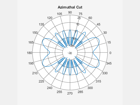

Generate Vertical Slice

Use the patternElevation function to compute the elevation pattern. Observe that the computation is quick, as expected for simulation at only 361 points for this 2-D slice.

theta = 0:360;
el = 90-theta;
tic
pE = patternElevation(ant,f,Elevation=el);
toc

Elapsed time is 1.252579 seconds.

Use the polarpattern function to visualize the calculated elevation pattern.

figure
polarpattern(el,pE,TitleTop="Elevation Cut")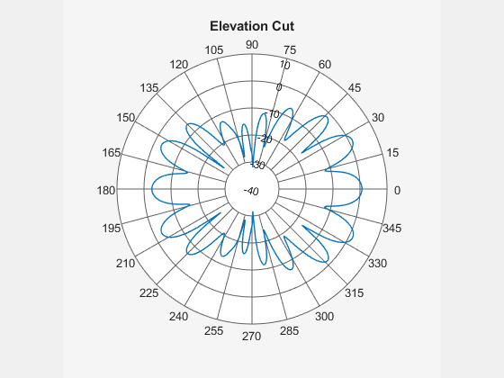

Examine Slice Data

Here are a few observations about the 2-D pattern slice data:

• There are many, finely-spaced side lobes, and the directivity pattern appears to have a complicated structure. It is not easy to discern how the 3-D pattern looks simply from the slices. This necessitates sophisticated reconstruction techniques to build the full, 3-D pattern.

• The main radiation lobes and maximum directivity are not along the boresight direction, namely the positive x-axis or $\left(\varphi ,\theta \right)=\left(0°,90°\right)$. This violates a key assumption of many of the analytical methods, such as those utilized by the patternFromSlices function, rendering them ineffective.

• Radiation is similarly as strong in the backplane as it is in the frontplane, and so the backplane data is important and cannot be ignored or discarded. However, many of the existing reconstruction techniques prioritize the frontplane data and deemphasize or do not even account for the backplane data in one or both slices.

Reconstruct and Visualize 3-D Pattern Using Deep Learning

Use the patternFromAI function to predict the 3-D pattern using a deep-learning-based approach. Note that this step does not involve any full-wave electromagnetic simulation.

tic
[pR,thetaR,phiR] = patternFromAI(pE,theta,pA,phi);
toc

Elapsed time is 11.705783 seconds.

Use the patternCustom function to visualize the reconstructed pattern. Alternatively, you can call the patternFromAI function without any output arguments to directly visualize the reconstructed pattern. Observe that reconstruction is relatively quick due to the fast inference time of the pretrained network.

figure
patternCustom(pR,thetaR,phiR)
title("Reconstructed 3-D Pattern—Deep Learning Model")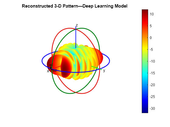

Compute and Visualize 3-D Pattern Using Full-Wave Simulation

Use the pattern function to perform full-wave electromagnetic simulation to compute the 3-D pattern of the rhombic antenna. Note here that the elevation angles span only a 180° range to avoid redundancy in the spatial locations or angular directions, given that the azimuthal angles also span a 360° range. Observe that the computation is time-consuming due to the dense angular resolution: 361×181 points.

azR = phiR;
elR = 90-thetaR;
tic
p0 = pattern(ant,f,azR,elR);
toc

Elapsed time is 63.415948 seconds.

Use the patternCustom function to visualize the pattern data. Prior to doing so, transpose the output returned by the pattern function so that it is of size M-by-N, where M=numel(az) and N=numel(el). This is to facilitate direct comparison with the prediction made by the patternFromAI function, whose returned output is also of size M-by-N.

p0 = p0.';
assert(isequal(size(pR),size(p0)))

figure
patternCustom(p0,thetaR,phiR)
title("Actual 3-D Pattern—Full-Wave Simulation")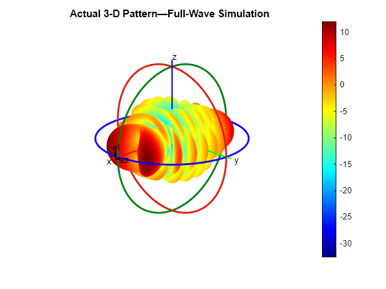

Compare Predicted vs. Actual 3-D Patterns

This example utilizes several visualization techniques and statistical metrics to compare the predicted (reconstructed) pattern from the deep learning model vs. the actual (simulated) pattern from numerical solution. Note that the actual pattern would generally not be available as a reference or "ground truth" for comparison, as the intention is to rely on the deep learning model's prediction as a reliable replacement for full 3-D pattern measurement or full-wave simulation. That said, the purpose of this example is to demonstrate that the patternFromAI function is capable of achieving strong reconstruction accuracy for antennas whose patterns are of high complexity. Thus, it makes comparisons against the ground truth.

Visualize Patterns Side-by-Side in Rectangular Coordinate System

Examine and compare the 3-D patterns as plotted in the rectangular coordinate system. As with the pattern plots seen earlier in the spherical coordinate system, the predicted and actual 3-D patterns are nearly indistinguishable upon visual comparison.

figure
tiledlayout(1,2)
nexttile
helperPatternCustomRectangular(pR,thetaR,phiR,"Predicted Pattern")
nexttile
helperPatternCustomRectangular(p0,thetaR,phiR,"Actual Pattern")

Visualize Directional Distribution of Absolute Prediction Error

Use the patternCustom function to plot the absolute error in the rectangular coordinate system as a function of the two angular coordinates. Overall, the reconstruction accuracy is very good.

figure
pAbsErr = abs(pR-p0);
helperPatternCustomRectangular(pAbsErr,thetaR,phiR,"Absolute Error (dBi)")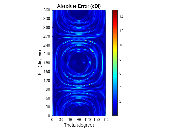

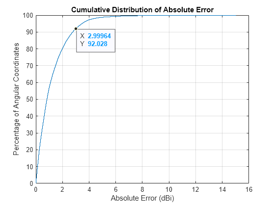
Create Cumulative Distribution Plot of Absolute Errors

Visualize the distribution of the errors in a cumulative distribution plot. Observe that the absolute prediction error is less than 3 dBi for nearly 90% of the angular coordinates.

pAbsErrSorted = sort(pAbsErr(:));
nAbsErr = numel(pAbsErrSorted);
pAbsErrCDF = (1:nAbsErr)./nAbsErr*100;

figure
hPlot = stairs(pAbsErrSorted,pAbsErrCDF);
xlabel("Absolute Error (dBi)")
ylabel("Percentage of Angular Coordinates")
title("Cumulative Distribution of Absolute Error")
grid on

idx = find(pAbsErrSorted<=3,1,"last");
[~] = datatip(hPlot,DataIndex=idx);

Quantify Overall Prediction Accuracy Using Statistical Error Metrics

Calculate the root-mean-squared error (RMSE) and mean absolute error (MAE) over the entire 3-D pattern to quantify the overall prediction error. Both metrics are in units of dBi.

errorRMSE = sqrt(mean(pAbsErr.^2,"all"))

errorRMSE = 1.8939

errorMAE = mean(pAbsErr,"all")

errorMAE = 1.4542

Supporting Functions

The following local function, helperPatternCustomRectangular, plots the angular distribution of the input quantity, such as directivity pattern or absolute error, in the rectangular coordinate system and configures some of the axes properties for display purposes.

function helperPatternCustomRectangular(p,theta,phi,titletext)
    patternCustom(p,theta,phi,CoordinateSystem="rectangular")
    title(titletext)
    view(2)
    colorbar
    xlim([-1,180])
    xticks(0:30:180)
    xtickangle(0)
    ylim([0,361])
    yticks(0:30:360)
    ytickangle(0)
    box on
end

References

[1] DiMeo, Peter, Sudarshan Sivaramakrishnan, and Vishwanath Iyer. “AI-Based 3D Antenna Pattern Reconstruction.” In 2024 IEEE International Symposium on Antennas and Propagation. Florence: IEEE, 2024.