Fading Channels
Overview of Fading Channels
Using Communications Toolbox™ you can implement fading channels using objects or blocks. Rayleigh and Rician fading channels are useful models of real-world phenomena in wireless communications. These phenomena include multipath scattering effects, time dispersion, and Doppler shifts that arise from relative motion between the transmitter and receiver. This section gives a brief overview of fading channels and describes how to implement them using the toolbox.
This figure depicts direct and major reflected paths between a stationary radio transmitter and a moving receiver. The shaded shapes represent reflectors such as buildings.
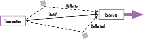
The major paths result in the arrival of delayed versions of the signal at the receiver. In addition, the radio signal undergoes scattering on a local scale for each major path. Such local scattering typically results from reflections off objects near the mobile. These irresolvable components combine at the receiver and cause a phenomenon known as multipath fading. Due to this phenomenon, each major path behaves as a discrete fading path. Typically, the fading process is characterized by a Rayleigh distribution for a non line-of-sight path and a Rician distribution for a line-of-sight path.
The relative motion between the transmitter and receiver causes Doppler shifts. Local scattering typically comes from many angles around the mobile. This scenario causes a range of Doppler shifts, known as the Doppler spectrum. The maximum Doppler shift corresponds to the local scattering components whose direction exactly opposes the trajectory of the mobile.
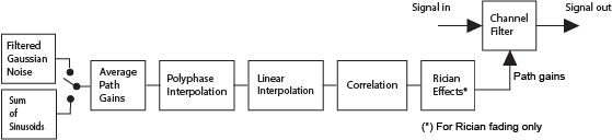
The channel filter applies path gains to the input signal, Signal in.
The path gains are computed by using either the Gaussian filtered noise or sum-of-sinusoids
method based on settings chosen in the fading channel object or block.
These blocks and objects enable you to model SISO or MIMO fading channels.
| Tool | SISO | MIMO |
|---|---|---|
| MATLAB® | ||
| Simulink® |
Implement Fading Channel Using an Object
A baseband channel model for multipath propagation scenarios that you implement using objects includes:
N discrete fading paths. Each path has its own delay and average power gain. A channel for which N = 1 is called a frequency-flat fading channel. A channel for which N > 1 is experienced as a frequency-selective fading channel by a signal of sufficiently wide bandwidth.
A Rayleigh or Rician model for each path.
Default channel path modeling using a Jakes Doppler spectrum, with a maximum Doppler shift that can be specified. Other types of Doppler spectra allowed (identical or different for all paths) include: flat, restricted Jakes, asymmetrical Jakes, Gaussian, bi-Gaussian, rounded, and bell.
If the maximum Doppler shift is set to 0 or omitted during the construction of a channel object, then the object models the channel as static. For this configuration, the fading does not evolve with time and the Doppler spectrum specified has no effect on the fading process.
Some additional information about typical values for delays and gains is in Choosing Realistic Channel Property Values.
Implement Fading Channel Using a Block
The Channels block library includes MIMO and SISO fading blocks that can simulate real-world phenomena in mobile communications. These phenomena include multipath scattering effects, in addition to Doppler shifts that arise from relative motion between the transmitter and receiver.
Tip
To model a channel that involves both fading and additive white Gaussian noise, use a fading channel block followed by an AWGN Channel block.
The MIMO Fading Channel and SISO Fading Channel blocks can be set to model Rayleigh or Rician fading distributions of the channel. Based on the type of signal path, choose the fading distribution to use.
| Signal Path | Fading Distribution |
|---|---|
| Direct line-of-sight path from transmitter to receiver | Rician |
| One or more major reflected paths from transmitter to receiver | Rayleigh |
You can use a single instance of a fading channel block configured for Rayleigh fading distribution to model multiple major reflected paths simultaneously.
Choosing appropriate block parameters for your situation is important. For more information, see Choosing Realistic Channel Property Values, and the MIMO Fading Channel and SISO Fading Channel block reference pages.
Visualize a Fading Channel
You can view the characteristics of a fading channel using channel visualization tools. For more information, see Channel Visualization.
Compensate for Fading Response
A communications system involving a fading channel usually requires components that compensate for the fading response. Typical approaches to compensate for fading include:
Differential modulation or a one-tap equalizer helps compensate for a frequency-flat fading channel. For information about implementing differential modulation, see the M-DPSK Modulator Baseband block reference page.
An equalizer with multiple taps helps compensate for a frequency-selective fading channel. See Equalization for more information.
The Adaptive Equalization with Filtering and Fading Channel example illustrates why compensating for a fading channel is necessary.
Methodology for Simulating Multipath Fading Channels
The Rayleigh and Rician multipath fading channel simulators in Communications Toolbox use the band-limited discrete multipath channel model of section 9.1.3.5.2 in [1]. This implementation assumes that the delay power profile and the Doppler spectrum of the channel are separable [1]. The multipath fading channel is therefore modeled as a linear finite impulse-response (FIR) filter. Let denote the set of samples at the input to the channel. Then the samples at the output of the channel are related to through:
where is the set of tap weights given by:
In the equations:
is the input sample period to the channel.
, where , is the set of path delays. K is the total number of paths in the multipath fading channel.
, where , is the set of complex path gains of the multipath fading channel. These path gains are uncorrelated with each other.
and are chosen so that is small when n is less than or greater than .
Two techniques, filtered Gaussian noise and sum-of-sinusoids, are used to generate the set of complex path gains, .
Each path gain process is generated by the following steps:
Filtered Gaussian Noise Technique
A complex uncorrelated (white) Gaussian process with zero mean and unit variance is generated in discrete time.
The complex Gaussian process is filtered by a Doppler filter with frequency response , where denotes the desired Doppler power spectrum.
The filtered complex Gaussian process is interpolated so that its sample period is consistent with the sample period of the input signal. A combination of linear and polyphase interpolation is used.
Sum-of-sinusoids Technique
Mutually uncorrelated Rayleigh fading waveforms are generated using the method described in [2], where i = 1 corresponds to the in-phase component and i = 2 corresponds to the quadrature component.
Where
Nk specifies the number of sinusoids used to model a single path.
is the discrete Doppler frequency and is calculated for each sinusoid component within a single path.
is the phase of the nth component of and is an i.i.d. random variable having a uniform distribution over the interval .
t is the fading process time.
When modeling a Jakes Doppler spectrum, the discrete Doppler frequencies, , with maximum shift fmax are given by
where
To advance the fading process in time, an initial time parameter, tinit, is introduced. The fading waveforms become
When tinit = 0, the fading process starts at time zero. A positive value of tinit advances the fading process relative to time zero while maintaining its continuity.
Channel fading samples are generated using the GMEDS1 [2] algorithm.
Calculate Complex Coefficients
The complex process resulting from either technique, , is scaled to obtain the correct average path gain. In the case of a Rayleigh channel, the fading process is obtained as:
where
In the case of a Rician channel, the fading process is obtained as:
where is the Rician K-factor of the kth path, is the Doppler shift of the line-of-sight component of the kth path (in Hz), and is the initial phase of the line-of-sight component of the kth path (in rad).
At the input to the band-limited multipath channel model, the transmitted symbols must be oversampled by a factor at least equal to the bandwidth expansion factor introduced by pulse shaping. For example, if sinc pulse shaping is used, for which the bandwidth of the pulse-shaped signal is equal to the symbol rate, then the bandwidth expansion factor is 1, and at least one sample per symbol is required at the input to the channel. If a raised cosine (RC) filter with a factor more than 1 is used, for which the bandwidth of the pulse-shaped signal is equal to twice the symbol rate, then the bandwidth expansion factor is 2, and at least two samples per symbol are required at the input to the channel.
Channel Filter Model Characteristics
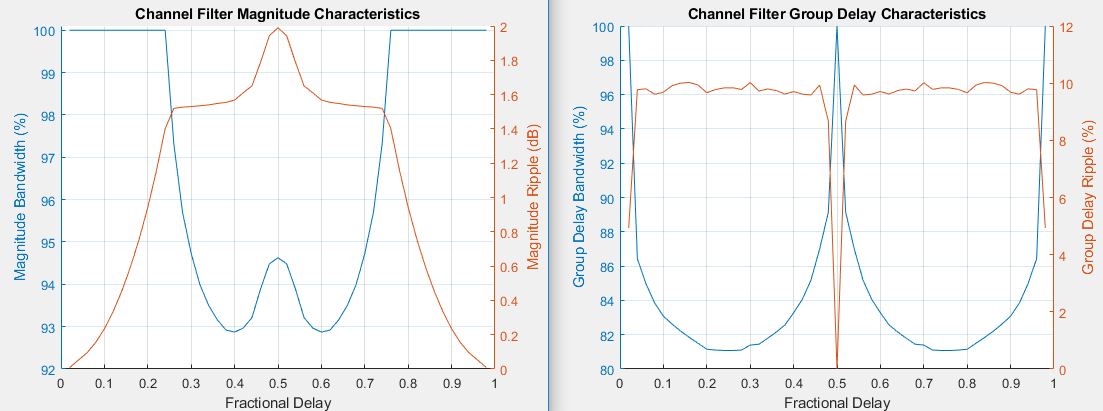
The channel filter implements a fractional delay (FD) finite impulse response (FIR) bandpass filter with a length of 16 coefficients for each candidate fractional delay at 0, 0.02, 0.04, …, 0.98.
Each discrete path is rounded to its nearest candidate fractional delay, so the delay error limit is 1% of the sample time. To achieve a group delay bandwidth exceeding 80% and a magnitude bandwidth exceeding 90%, the algorithm selects the optimal FIR coefficient values for each fractional delay, while satisfying the following criteria:
Group delay ripple ≤ 10%
Magnitude ripple ≤ 2 dB
Magnitude bandedge attenuation = 3 dB
The plots show bandwidths that satisfy the design criteria for group delay ripple, magnitude ripple, and magnitude bandedge attenuation.
References
[1] Jeruchim, M. C., Balaban, P., and Shanmugan, K. S., Simulation of Communication Systems, Second Edition, New York, Kluwer Academic/Plenum, 2000.
[2] Pätzold, Matthias, Cheng-Xiang Wang, and Bjorn Olav Hogstand. “Two New Sum-of-Sinusoids-Based Methods for the Efficient Generation of Multiple Uncorrelated Rayleigh Fading Waveforms.” IEEE Transactions on Wireless Communications. Vol. 8, Number 6, 2009, pp. 3122–3131.
Specify Fading Channels
Communications Toolbox models a fading channel as a linear FIR filter. Filtering a signal using a fading channel involves these steps:
Create a channel object that describes the channel that you want to use. A channel object is a type of MATLAB variable that contains information about the channel, such as the maximum Doppler shift.
Adjust properties of the channel object, if necessary, to tailor it to your needs. For example, you can change the path delays or average path gains.
Apply the channel object to your signal using calling the object.
This section describes how to define, inspect, and manipulate channel objects. The topics are:
Creating Channel Objects
To create a fading channel object suitable for your modeling situation, select one of these System objects.
| Function | Object | Situation Modeled |
|---|---|---|
| Rayleigh fading channel object | One or more major reflected paths | |
| Rician fading channel object | One direct line-of-sight path, possibly combined with one or more major reflected paths |
For example, this command creates a channel object representing a Rayleigh fading channel that acts on a signal sampled at 100,000 Hz. The maximum Doppler shift of the channel is 130 Hz.
rayChan1 = comm.RayleighChannel('SampleRate',1e5,...
               'MaximumDopplerShift',130); % Rayleigh fading channel object
To learn how to call the rayChan1 fading channel object to filter
the transmitted signal through the channel, see Using Fading Channels.
Duplicate and Copy Objects
You can also create another object by duplicating an existing object and then adjust
the properties of the new object, if necessary. To duplicate an object always use the
clone function such as:
rayChan2 = clone(rayChan1); % Copy rayChan1 to create an independent rayChan2.
instead of rayChan2 = rayChan1. The clone
command creates a copy of rayChan1 that is independent of
rayChan1. By contrast, the command rayChan2 =
rayChan1 creates rayChan2 as merely a reference to
rayChan1, so that rayChan1 and
rayChan2 always have indistinguishable content.
Displaying and Changing Object Properties
A channel object has numerous properties that record information about the channel model, about the state of a channel that has already filtered a signal, and about the channel operation on a future signal.
You can view the properties in these ways:
To view all properties of a channel object, enter the object name in the Command Window.
You can view a property of a channel object or assign the value to a variable by entering the object name followed by a dot (period), followed by the name of the property.
You can change the writable properties of a channel object in these ways:
To change the default value of a channel object property, enter the desired value in the object creation syntax.
To change the value of a writeable property of a channel object, issue an assignment statement that uses dot notation on the channel object. More specifically, dot notation means an expression that consists of the object name, followed by a dot, followed by the name of the property.
Display Rayleigh Channel Object Properties
Create a Rayleigh channel object and display the property values. Some of the properties values were assigned when the object was created, while other properties have default values. Retrieve the value of an individual property. For more information about specific channel properties, see the reference page for the comm.RayleighChannel object.
rayChan = comm.RayleighChannel( ...
    SampleRate=1e5, ...
    MaximumDopplerShift=130)
rayChan =
  comm.RayleighChannel with properties:

             SampleRate: 100000
     PathGainSampleRate: 'signal'
             PathDelays: 0
       AveragePathGains: 0
     NormalizePathGains: true
    MaximumDopplerShift: 130
        DopplerSpectrum: [1×1 struct]
       ChannelFiltering: true
    PathGainsOutputPort: false

  Show all properties
g = rayChan.AveragePathGains
g =
0
Adjust Rician Channel Object Properties
A Rician fading channel object has an additional property that does not appear for a Rayleigh fading channel object, namely, a scalar KFactor property. For more information about Rician channel properties, see the reference page for the comm.RicianChannel object.
Change Rician Channel Object Properties
Create a Rician channel object. Change the default setting for the Visualization property from 'Off' to 'Impulse response' to generate an impulse response plot of the output signal when the object is called. The output displays a subset of all the properties of the channel object. Select all properties to see the complete set of properties for ricChan.
ricChan= comm.RicianChannel;
ricChan.Visualization = 'Impulse response'
ricChan =
comm.RicianChannel with properties:
SampleRate: 1
PathGainSampleRate: 'signal'
PathDelays: 0
AveragePathGains: 0
NormalizePathGains: true
KFactor: 3
DirectPathDopplerShift: 0
DirectPathInitialPhase: 0
MaximumDopplerShift: 1.0000e-03
DopplerSpectrum: [1×1 struct]
ChannelFiltering: true
PathGainsOutputPort: false
Show all properties
Relationships Among Channel Object Properties
Some properties of a channel object are related to each other such that when one
property's value changes, another property's value must change in some corresponding way
to keep the channel object consistent. For example, if you change the vector length of
PathDelays, then the value of AveragePathGains
must change so that its vector length equals that of the new value of
PathDelays. This is because the length of each of the two vectors
equals the number of discrete paths of the channel. For details about linked properties
and an example, see comm.RayleighChannel or comm.RicianChannel.
Specify Doppler Spectrum of Fading Channel
The Doppler spectrum of a channel object is specified through its
DopplerSpectrum property. The value of this property must be either:
A Doppler spectrum structure. In this case, the same Doppler spectrum applies to each path of the channel object.
A cell array of Doppler spectrum structures of the same length as the
PathDelaysvector property. In this case, the Doppler spectrum of each path is given by the corresponding Doppler spectrum structure in the vector.When the vector length of the
PathDelaysproperty is increased, the length ofDopplerSpectrumis automatically increased to match the length ofPathDelays, by appending Jakes Doppler spectrum structures.If the length of the
PathDelaysvector property is decreased, the length ofDopplerSpectrumis automatically decreased to match the length ofPathDelays, by removing the last Doppler spectrum structures.
A Doppler spectrum structure contains the properties used to characterize the
Doppler spectrum, but the maximum Doppler shift is a property of the channel object. This
section describes how to create and manipulate Doppler spectrum structures, and how to
assign them to the DopplerSpectrum property of channel objects.
Create a Doppler Spectrum Structure
To create Doppler spectrum structures, use the doppler function. The sole purpose of the doppler function is to create Doppler spectrum structures used to specify
the value of the DopplerSpectrum property of channel objects. Select
from the following:
doppler('Jakes')doppler('Flat')doppler('Rounded', ...)doppler('Bell', ...)doppler('Asymmetric Jakes', ...)doppler('Restricted Jakes', ...)doppler('Gaussian', ...)doppler('BiGaussian', ...)
For example, a Gaussian spectrum with a normalized (by the maximum Doppler shift of the channel) standard deviation of 0.1, can be created as:
dopp1 = doppler('Gaussian',0.1);Note
When creating a Doppler spectrum structure, consider the following dependencies:
If you assign a single Doppler spectrum structure to
DopplerSpectrum, all paths have the same specified Doppler spectrum.If the
FadingTechniqueproperty is'Sum of sinusoids',DopplerSpectrummust bedoppler('Jakes');If you assign a row cell array of different Doppler spectrum structures to
DopplerSpectrum, each path has the Doppler spectrum specified by the corresponding structure in the cell array. In this case, the length ofDopplerSpectrummust be equal to the length ofPathDelays.To generate C code, specify
DopplerSpectrumto a single Doppler spectrum structure.
View and Change Doppler Spectrum Structure Properties
Create a Doppler spectrum structure by specifying the type of Doppler spectrum as 'Rounded', then modify settings of the polynomial type.
A rounded Doppler spectrum structure with default properties is created and displayed, and the third element of the Polynomial field is modified.
doppRound = doppler('Rounded')doppRound = struct with fields:
SpectrumType: 'Rounded'
Polynomial: [1 -1.7200 0.7850]
Adjust the third coefficient of the polynomial.
doppRound.Polynomial(3) = 0.825
doppRound = struct with fields:
    SpectrumType: 'Rounded'
      Polynomial: [1 -1.7200 0.8250]
Be aware that it is possible to modify a Doppler spectrum structure to an invalid configuration. Validation of the Doppler spectrum structure settings is performed when the structure is used by a fading channel object. The doppRound spectrum structure defined above is valid.
ricianCh = comm.RicianChannel('DopplerSpectrum',doppRound)ricianCh =
comm.RicianChannel with properties:
SampleRate: 1
PathGainSampleRate: 'signal'
PathDelays: 0
AveragePathGains: 0
NormalizePathGains: true
KFactor: 3
DirectPathDopplerShift: 0
DirectPathInitialPhase: 0
MaximumDopplerShift: 1.0000e-03
DopplerSpectrum: [1×1 struct]
ChannelFiltering: true
PathGainsOutputPort: false
Show all properties
Use Doppler Spectrum Structures Within Channel Objects
The DopplerSpectrum property of a channel object can be changed by
assigning to it a Doppler spectrum structure or a vector of Doppler spectrum structures.
Create Rayleigh Channel with Flat Doppler Spectrum
This example shows how to change the default Jakes Doppler spectrum of a configured Rayleigh channel object to a flat Doppler spectrum.
Create a Rayleigh Channel Object
Set the sample rate to 9600 Hz and the maximum Doppler shift to 100 Hz.
rayChan = comm.RayleighChannel( ...
    'SampleRate',9600,'MaximumDopplerShift',100)
rayChan =
  comm.RayleighChannel with properties:

             SampleRate: 9600
     PathGainSampleRate: 'signal'
             PathDelays: 0
       AveragePathGains: 0
     NormalizePathGains: true
    MaximumDopplerShift: 100
        DopplerSpectrum: [1×1 struct]
       ChannelFiltering: true
    PathGainsOutputPort: false

  Show all properties
rayChan.DopplerSpectrum
ans = struct with fields:
    SpectrumType: 'Jakes'
Modify the Doppler Spectrum
Create a flat Doppler spectrum structure, and then assign it in the rayChan object.
doppFlat = doppler('Flat')doppFlat = struct with fields:
SpectrumType: 'Flat'
rayChan.DopplerSpectrum = doppFlat
rayChan =
  comm.RayleighChannel with properties:

             SampleRate: 9600
     PathGainSampleRate: 'signal'
             PathDelays: 0
       AveragePathGains: 0
     NormalizePathGains: true
    MaximumDopplerShift: 100
        DopplerSpectrum: [1×1 struct]
       ChannelFiltering: true
    PathGainsOutputPort: false

  Show all properties
rayChan.DopplerSpectrum
ans = struct with fields:
    SpectrumType: 'Flat'
Create Rician Channel with Gaussian Doppler Spectrum
This example shows how to change the default Jakes Doppler spectrum of a configured Rician channel object to a Gaussian Doppler spectrum with normalized standard deviation of 0.3. Then, display the DopplerSpectrum property and change the normalized standard deviation of the Doppler spectrum to 1.1.
Create a Rician Channel Object
Set the sample rate to 9600 Hz, the maximum Doppler shift to 100 Hz, and K factor to 2.
ricChan = comm.RicianChannel( ...
    'SampleRate',9600,'MaximumDopplerShift',100,'KFactor',2)
ricChan =
  comm.RicianChannel with properties:

                SampleRate: 9600
        PathGainSampleRate: 'signal'
                PathDelays: 0
          AveragePathGains: 0
        NormalizePathGains: true
                   KFactor: 2
    DirectPathDopplerShift: 0
    DirectPathInitialPhase: 0
       MaximumDopplerShift: 100
           DopplerSpectrum: [1×1 struct]
          ChannelFiltering: true
       PathGainsOutputPort: false

  Show all properties
ricChan.DopplerSpectrum
ans = struct with fields:
    SpectrumType: 'Jakes'
Modify the Doppler Spectrum
Create a Gaussian Doppler spectrum structure with normalized standard deviation of 0.3 and assign it in the ricChan object.
doppGaus = doppler('Gaussian',0.3)doppGaus = struct with fields:
SpectrumType: 'Gaussian'
NormalizedStandardDeviation: 0.3000
ricChan.DopplerSpectrum = doppGaus
ricChan =
  comm.RicianChannel with properties:

                SampleRate: 9600
        PathGainSampleRate: 'signal'
                PathDelays: 0
          AveragePathGains: 0
        NormalizePathGains: true
                   KFactor: 2
    DirectPathDopplerShift: 0
    DirectPathInitialPhase: 0
       MaximumDopplerShift: 100
           DopplerSpectrum: [1×1 struct]
          ChannelFiltering: true
       PathGainsOutputPort: false

  Show all properties
ricChan.DopplerSpectrum
ans = struct with fields:
                   SpectrumType: 'Gaussian'
    NormalizedStandardDeviation: 0.3000
ricChan.DopplerSpectrum.NormalizedStandardDeviation = 1.1;
ricChan.DopplerSpectrum
ans = struct with fields:
                   SpectrumType: 'Gaussian'
    NormalizedStandardDeviation: 1.1000
Create Rayleigh Channel Using Independent Doppler Spectrum
Change the default Jakes Doppler spectrum of a configured three-path Rayleigh channel object to a cell array of different Doppler spectra, and then change the properties of the Doppler spectrum of the third path.
Create a Rayleigh Channel Object
Set the sample rate to 9600 Hz, the maximum Doppler shift to 100 Hz, and specify path delays of 0, 1e-4, and 2.1e-4 seconds.
rayChan = comm.RayleighChannel( ...
    SampleRate=9600, ...
    MaximumDopplerShift=100, ...
    PathDelays=[0 1e-4 2.1e-4])
rayChan =
  comm.RayleighChannel with properties:

             SampleRate: 9600
     PathGainSampleRate: 'signal'
             PathDelays: [0 1.0000e-04 2.1000e-04]
       AveragePathGains: 0
     NormalizePathGains: true
    MaximumDopplerShift: 100
        DopplerSpectrum: [1×1 struct]
       ChannelFiltering: true
    PathGainsOutputPort: false

  Show all properties
rayChan.DopplerSpectrum
ans = struct with fields:
    SpectrumType: 'Jakes'
Modify the Doppler Spectrum
Specify the DopplerSpectrum property as a cell array with an independent Doppler spectrum for each path.
rayChan.DopplerSpectrum = ...
    {doppler('Flat') doppler('Flat') doppler('Rounded')}
rayChan =
  comm.RayleighChannel with properties:

             SampleRate: 9600
     PathGainSampleRate: 'signal'
             PathDelays: [0 1.0000e-04 2.1000e-04]
       AveragePathGains: 0
     NormalizePathGains: true
    MaximumDopplerShift: 100
        DopplerSpectrum: {[1×1 struct]  [1×1 struct]  [1×1 struct]}
       ChannelFiltering: true
    PathGainsOutputPort: false

  Show all properties
rayChan.DopplerSpectrum{:}ans = struct with fields:
SpectrumType: 'Flat'
ans = struct with fields:
    SpectrumType: 'Flat'
ans = struct with fields:
SpectrumType: 'Rounded'
Polynomial: [1 -1.7200 0.7850]
Change the Polynomial property for the third path.
rayChan.DopplerSpectrum{3}.Polynomial = [1 -1.21 0.7]rayChan =
comm.RayleighChannel with properties:
SampleRate: 9600
PathGainSampleRate: 'signal'
PathDelays: [0 1.0000e-04 2.1000e-04]
AveragePathGains: 0
NormalizePathGains: true
MaximumDopplerShift: 100
DopplerSpectrum: {[1×1 struct] [1×1 struct] [1×1 struct]}
ChannelFiltering: true
PathGainsOutputPort: false
Show all properties
rayChan.DopplerSpectrum{:}ans = struct with fields:
SpectrumType: 'Flat'
ans = struct with fields:
    SpectrumType: 'Flat'
ans = struct with fields:
    SpectrumType: 'Rounded'
      Polynomial: [1 -1.2100 0.7000]
Configure Channel Objects
Before you filter a signal using a channel object, make sure that the properties of the channel have suitable values for the situation you want to model. This section offers some guidelines to help you choose realistic values that are appropriate for your modeling needs. The topics are
The syntaxes for viewing and changing values of properties of channel objects are described in Specifying a Fading Channel.
Choose Realistic Channel Property Values
Here are some tips for choosing property values that describe realistic channels:
Path Delays
By convention, the first delay is typically set to zero. The first delay corresponds to the first arriving path.
For indoor environments, path delays after the first are typically between 1e-9 seconds and 1e-7 seconds.
For outdoor environments, path delays after the first are typically between 1e-7 seconds and 1e-5 seconds. Large delays in this range might correspond, for example, to an area surrounded by mountains.
The ability of a signal to resolve discrete paths is related to its bandwidth. If the difference between the largest and smallest path delays is less than about 1% of the symbol period, then the signal experiences the channel as if it had only one discrete path.
Average Path Gains
The average path gains in the channel object indicate the average power gain of each fading path. In practice, an average path gain value is a large negative dB value. However, computer models typically use average path gains in the range of [-20, 0] dB.
The dB values in a vector of average path gains often decay roughly linearly as a function of delay, but the specific delay profile depends on the propagation environment.
To ensure that the expected total power of the combined path gains is 1, you can normalize path gains via the
NormalizePathGainsproperty of the channel object.
Maximum Doppler Shifts
Doppler shifts are specified in terms of the relative speed between a transmitter and a receiver. The maximum Doppler shift in Hertz, fd = vf ∕ c. In the formula, v is the relative speed in m/s, f is the transmission carrier frequency in Hertz, and c is the speed of light (3×10⁸ m/s). The relative speed is a magnitude with no directional information.
Apply the maximum Doppler shift formula assuming a transmission carrier frequency of 900 MHz, a car moving at freeway speed, and a walking pedestrian. A signal transmitted from a car moving at freeway speed to a stationary receiver would experience a maximum Doppler shift of approximately 80 Hz. A signal transmitted from a mobile held by a walking pedestrian to a stationary receiver would experience a maximum Doppler shift of approximately 4 Hz.
A maximum Doppler shift of 0 corresponds to a static channel that comes from a Rayleigh or Rician distribution.
Doppler Spectrum
K-Factor for Rician Fading Channels
The Rician K-factor specifies the ratio of specular-to-diffuse power for a direct line-of-sight path. The ratio is expressed linearly, not in dB.
For Rician fading, the K-factor is typically in the range [1, 10].
A K-factor of 0 corresponds to Rayleigh fading.
Line-of-Sight (LOS) Path Doppler Shift for Rician Fading Channels
The Rician LOS path Doppler shift, also known as direct path Doppler shift, specifies the relative motion of the LOS path between a transmitter and a receiver.
The Rician LOS path Doppler shift in Hertz, fd_los = (u⋅w) × f ∕ c. In the formula, (u⋅w) is the dot product of vectors u and w, u is the normalized LOS path from the transmitter to the receiver, w is the velocity of the receiver relative to transmitter, f is the transmission carrier frequency in Hertz, and c is the speed of light (3×10⁸ m/s).
Apply this formula for a transmission carrier frequency of 900 MHz at a specified relative velocity. For a signal from a transmitter at the coordinate origin that reaches a receiver at the coordinate [100 100 0], where the relative velocity between the transmitter and receiver w = [3 -6 0.1].
f = 9e8;                          % 900 MHz
c = physconst('LightSpeed');
u1 = [0 0 0];                     % Transmitter coordinates in meters
u2 =  [100 100 0];                % Receiver coordinates in meters
u = u2 - u1;
uNormalized = u/norm(u);
w = [3 -6 0.1];                   % Receiver velocity, m/s
fd_los = uNormalized * w' * f / c % Doppler shift, Hz
fd_los =
   -6.3684
Doppler Spectrum Parameters
See the
dopplerreference page for the respective Doppler spectrum structures for descriptions of the parameters and their significance.
Configure Channel Objects Based on Simulation Needs
Tips for configuring a channel object to customize the filtering process:
If your data is partitioned into a series of vectors (that you process within a loop, for example), you can call the channel object multiple times (in each iteration within a loop). The state information of the channel is updated and saved after each invocation. The channel output is irrelevant to how the data is partitioned (vector length).
If want the channel output to be repeatable, choose the seed option for the
RandomStreamproperty of the channel object. To repeat the output, call theresetobject function to reset both the internal filters and the internal random number generator.If you want to model discontinuously transmitted data, set the
FadingTechniqueproperty to'Sum of sinusoids'and theInitialTimeSourceproperty to'Input port'for the channel object. When calling the object, specify the start time of each data vector/frame to be processed by the channel via an input.If you want to normalize the fading process so that the expected value of the path gains' total power is 1 (the channel does not contribute additional power gain or loss), set the
NormalizePathGainsproperty of the channel object totrue.
Use Fading Channels
After you have created a channel object as described in Specifying a Fading Channel, you can call the object to pass a signal through the channel. Provide the signal as an input argument to the channel object. At the end of the filtering operation, the channel object retains its state so that you can find out the final path gains or the total number of samples that the channel has processed by calling the info object function with the object as the input argument.
For an example that illustrates the basic syntax and state retention, see Power of a Faded Signal.
To visualize the characteristics of the channel, set the
Visualization property to 'Impulse response',
'Frequency response', or 'Doppler spectrum'. For
more information, see Channel
Visualization.
Visualize Three-Path Rayleigh Channel
Visualize the impulse response of a channel.
Create a channel object
While creating the channel object, use name-value pairs to set the Visualization property to 'Impulse response'.
rayChan = comm.RayleighChannel( ...
    SampleRate=100000, ...
    MaximumDopplerShift=130,...
    PathDelays=[0 1.5e-5 3.2e-5], ...
    AveragePathGains=[0, -3, -3], ...
    Visualization='Impulse response');
Generate a bit stream and create a DBPSK modulator object. Modulate the bit stream and pass the modulated DBPSK signal through the channel by calling the channel object. The impulse response is plotted when the object is called.
tx = randi([0 1],500,1);
dbspkMod = comm.DBPSKModulator;
dpskSig = dbspkMod(tx);
y = rayChan(dpskSig);
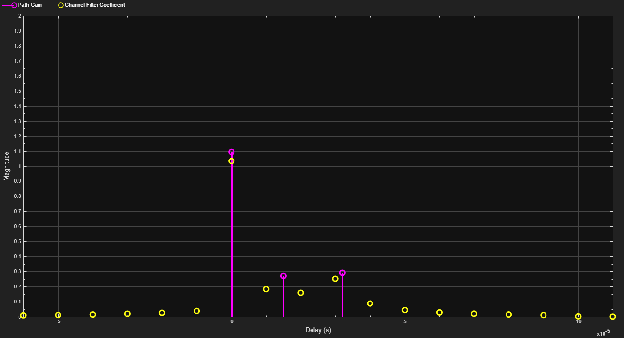
Rayleigh Fading Channel
These examples use fading channels:
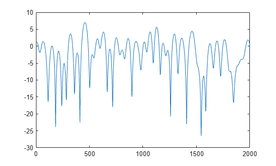
Power of Faded Signal
Plot the power of a faded signal versus sample number. The example illustrates the syntax of creating and calling a comm.RayleighChannel fading channel object, and the state retention of the channel object.
rayChan = comm.RayleighChannel( ...
    SampleRate=10000, ...
    MaximumDopplerShift=100);
sig = 1i*ones(2000,1);
out = rayChan(sig);
rayChan
rayChan =
  comm.RayleighChannel with properties:

             SampleRate: 10000
     PathGainSampleRate: 'signal'
             PathDelays: 0
       AveragePathGains: 0
     NormalizePathGains: true
    MaximumDopplerShift: 100
        DopplerSpectrum: [1×1 struct]
       ChannelFiltering: true
    PathGainsOutputPort: false

  Show all properties
Plot power of faded signal, versus sample number.
plot(20*log10(abs(out)))
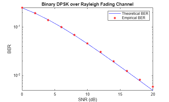
DBPSK Empirical Versus Theoretical Performance in Fading Conditions
This example creates a frequency-flat Rayleigh fading channel object and calls it to process a DBPSK signal consisting of a single vector. The bit error rate (BER) is computed for different values of the signal-to-noise ratio (SNR). When applying channel impairments, the fading channel filter can be applied before the loop on SNR values. Since the AWGN must account for the signal to noise ratio (SNR), the signal is passed through the AWGN channel filter later, inside the loop over SNR values. This sequence is recommended when you combine fading with AWGN.
Create modulator, demodulator, Rayleigh fading channel, AWGN channel, and an error rate calculator System objects to use for the simulation.
mod = comm.DBPSKModulator;
demod = comm.DBPSKDemodulator;
chan = comm.RayleighChannel( ...
    SampleRate=1e4, ...
    MaximumDopplerShift=100);
awgnChan = comm.AWGNChannel( ...
    NoiseMethod='Signal to noise ratio (SNR)');
errorCalc = comm.ErrorRate;
Generate a random bit stream of symbols and apply DBPSK modulation to the symbols. Pass the DBPSK modulated data through the fading channel.
M = 2;                       % DBPSK modulation order
tx = randi([0 M-1],50000,1); % Generate a random bit stream

dpskSig = mod(tx);
fadedSig = chan(dpskSig);
Preallocate a vector for BER results. Compute the error rate for different values of SNR.
SNR = 0:2:20;
numSNR = length(SNR);
berVec = zeros(3, numSNR);

for n = 1:numSNR
   awgnChan.SNR = SNR(n);
   rxSig = awgnChan(fadedSig);
   rx = demod(rxSig);
   reset(errorCalc)

   berVec(:,n) = errorCalc(tx,rx);
end
BER = berVec(1,:);
Compute theoretical performance results, for comparison.
BERtheory = berfading(SNR,'dpsk',M,1);Plot BER results.
semilogy(SNR,BERtheory,'b-',SNR,BER,'r*');
legend('Theoretical BER','Empirical BER');
xlabel('SNR (dB)');
ylabel('BER');
title('Binary DPSK over Rayleigh Fading Channel');
Work with Channel Filter Delays
To compare input and output data sets directly, you must account for the delay by using appropriate truncating or padding operations. The fading channel object's ChannelFilterDelay property value represents the number of samples of lag between the output of the channel and the input. This example illustrates a way to account for the delay while computing a bit error rate.
Create DBPSK modulator, DBPSK demodulator, fading channel, and error rate calculation System objects to use for the simulation. Retrieve the ChannelFilterDelay property by using the info object function. Configure the error rate calculation object to account for the fading channel output delay.
bitRate = 50000;
mod = comm.DBPSKModulator;
demod = comm.DBPSKDemodulator;
rayChan = comm.RayleighChannel( ...
    SampleRate=bitRate, ...
    MaximumDopplerShift=4, ...
    PathDelays=[0 0.5/bitRate], ...
    AveragePathGains=[0 -10]);
chInfo = info(rayChan);
delay = chInfo.ChannelFilterDelay
delay =
7
errorCalc = comm.ErrorRate(ReceiveDelay=delay);
Generate random data symbols for DBPSK modulation. Generate DBPSK modulated data, pass the modulated data through the fading channel, and demodulate the channel impaired data.
M = 2;                       % DBPSK modulation order
tx = randi([0 M-1],50000,1);
dpskSig = mod(tx);
fadedSig = rayChan(dpskSig);
rx = demod(fadedSig);
Compute and display bit error rate statistics. The error rate calculation object configuration accounts for the expected fading channel output delay.
berVec = errorCalc(tx,rx);
sprintf(['%d bits were received.\nThere were %d bits ' ...
    'in error.\nThe computed BER is %1.2f.'], ...
    berVec(3), berVec(2), berVec(1))
ans =
    '49993 bits were received.
     There were 737 bits in error.
     The computed BER is 0.01.'
Channel Filtering Using For Loop
This example filters input data through a Rayleigh fading channel within a for loop. It uses the small data sets from successive iterations to create an animated effect. The Rayleigh fading channel has two discrete major paths. For information on filtering data through a channel multiple times while maintaining continuity from one invocation to the next, see Configure Channel Objects Based on Simulation Needs.
Set up parameters. Specify a bit rate of 50e3 Hz, and a loop iteration count of 125. Create Rayleigh fading channel, and constellation diagram System objects.
bitRate = 50000;   % Data rate is 50 kb/s
numTrials = 125;   % Number of iterations of loop
M = 4;             % QPSK modulation order
phaseoffset = pi/4
phaseoffset =
0.7854
rayChan = comm.RayleighChannel( ...
    SampleRate=bitRate, ...
    MaximumDopplerShift=4, ...
    PathDelays=[0 2e-5], ...
    AveragePathGains=[0 -9]);
cd = comm.ConstellationDiagram;
Plot the expected ideal constellation by using the PlotConstellation property of the pskmod function. Generate random symbols, apply QPSK modulation to the symbols, and pass the modulated signal through the fading channel in a loop, maintaining continuity. Plot only the current data in each iteration.
pskmod([0 M-1],M,phaseoffset,PlotConstellation=true);
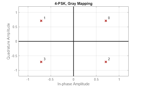
for n = 1:numTrials
   tx = randi([0 M-1],500,1);
   pskSig = pskmod(tx,M,phaseoffset);
   fadedSig = rayChan(pskSig);

   % Plot the new data for each for loop iteration.
   update(cd,fadedSig);
end

Rician Fading Channel
Quasi-Static Channel Modeling
Typically, a path gain in a fading channel changes insignificantly over a period of 1/(100fd) seconds, where fd is the maximum Doppler shift. Because this period corresponds to a very large number of bits in many modern wireless data applications, assessing performance over a statistically significant range of channel fading requires simulating a prohibitively large amount of data. This example illustrates the quasi-static channel modeling approach to gathering a statistically significant number of errors. Quasi-static channel modeling provides a more tractable approach, which you can implement using these steps:
Generate a random channel realization using a maximum Doppler shift of 0.
Process some large number of bits.
Compute error statistics.
Repeat these steps many times to produce a distribution of the performance metric.
Set simulation variables for bits per trial, number of trials (specifically the number of packets), and the modulation order. Typically, numTrials would be a large number to get an accurate estimate of outage probabilities or packet error rate. Use 20 here just to make the example run more quickly. Create modulator, demodulator, and Rician channel System objects. Set the maximum Doppler shift to zero for the Rician channel.
numBits = 10000; % Each trial uses 10000 bits
numTrials = 20;  % Number of BER computations
M = 4;

dpskMod = comm.DPSKModulator(ModulationOrder=M);
dpskDemod = comm.DPSKDemodulator(ModulationOrder=M);
ricianChan = comm.RicianChannel(KFactor=3,MaximumDopplerShift=0);
Within a for loop, generate a random bit stream, DPSK modulate the signal, filter the modulated signal through a Rician fading and AWGN channels, and demodulate the faded signal. For the symbol error rate (SER), begin the computation on each packet at sample 2, ignoring the first sample because of DPSK initial condition.
nErrors = zeros(1,numTrials);
for n = 1:numTrials
   tx = randi([0 M-1],numBits,1);
   dpskSig = dpskMod(tx);
   fadedSig = ricianChan(dpskSig);
   rxSig = awgn(fadedSig,15,'measured');
   rx = dpskDemod(rxSig);
   nErrors(n) = symerr(tx(2:end),rx(2:end));
end
Display the nErrors vector, which contains the number of symbol errors per packet. Compute the packet error rate. Run to run results vary due to randomness in the example.
nErrors(1:10)
ans = 1×10

     0     1     0     0     1     0     0     0     0     0
nErrors(11:20)
ans = 1×10

     0     0     0     1     0     0     0     1     0     0
per = mean(nErrors > 0) % Packet error rateper = 0.2000
More About the Quasi-Static Technique
As an example to show how the quasi-static channel modeling approach can save computation, consider a wireless local area network (LAN) in which the carrier frequency is 2.4 GHz, mobile speed is 1 m/s, and bit rate is 10 Mb/s. The following expression shows that the channel changes insignificantly over 12,500 bits:
A traditional Monte Carlo approach for computing the error rate of this system would entail simulating thousands of times, totalling tens of millions of bits. By contrast, a quasi-static channel modeling approach would simulate a few packets at each of about 100 locations to arrive at a spatial distribution of error rates. From this distribution one could determine, for example, how reliable the communication link is for a random location within the indoor space. If each simulation contains 5,000 bits, 100 simulations would process half a million bits in total. This is substantially fewer bits compared to the traditional Monte Carlo approach.