sigma
Singular values of frequency response of dynamic system
Description
[ returns the singular values
sv,wout]
= sigma(sys)sv of the frequency response of dynamic system model
sys at each frequency in the vector wout. The
function automatically determines frequencies to plot based on system dynamics.
sigma(___) plots the singular values of the frequency
response of sys with default plotting options for all of the previous
input argument combinations. If sys is a single-input, single-output
(SISO) model, then the singular value plot is similar to its Bode magnitude response. For
more plot customization options, use sigmaplot.
To plot singular values for multiple dynamic systems on the same plot, you can specify
sysas a comma-separated list of models. For example,sigma(sys1,sys2,sys3)plots the singular values for three models on the same plot.To specify a color, line style, and marker for each system in the plot, specify a
LineSpecvalue for each system. For example,sigma(sys1,LineSpec1,sys2,LineSpec2)plots two models and specifies their plot style. For more information on specifying aLineSpecvalue, seesigmaplot.
Examples
Create a singular value plot of the following continuous-time SISO dynamic system.
H = tf([1 0.1 7.5],[1 0.12 9 0 0]);
sigma(H)

sigma automatically selects the plot range based on the system dynamics.
Create a singular value plot over a specified frequency range. Use this approach when you want to focus on the dynamics in a particular range of frequencies.
H = tf([-0.1,-2.4,-181,-1950],[1,3.3,990,2600]);
sigma(H,{1,100})
grid on
The cell array {1,100} specifies the minimum and maximum frequency values in the plot. When you provide frequency bounds in this way, the function selects intermediate points for frequency response data.
Alternatively, specify a vector of frequency points to use for evaluating and plotting the frequency response.
w = [1 5 10 15 20 23 31 40 44 50 85 100];
sigma(H,w,'.-')
grid on
sigma plots the frequency response at the specified frequencies only.
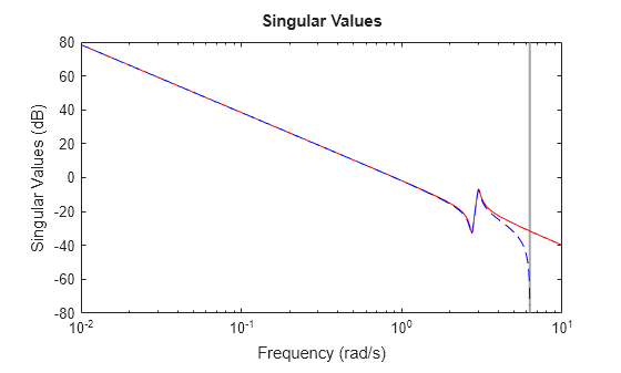
Compare the frequency response of a continuous-time system to an equivalent discretized system on the same singular value plot.
Create continuous-time and discrete-time dynamic systems.
H = tf([1 0.1 7.5],[1 0.12 9 0 0]);
Hd = c2d(H,0.5,'zoh');
Create a plot that displays both systems.
sigma(H,Hd)
legend("Continuous","Discrete")

The sigma plot of a discrete-time system includes a vertical line marking the Nyquist frequency of the system.
Specify the line style, color, or marker for each system in a sigma plot using the LineSpec input argument.
H = tf([1 0.1 7.5],[1 0.12 9 0 0]);
Hd = c2d(H,0.5,'zoh');
sigma(H,'r',Hd,'b--')
The first LineSpec, 'r', specifies a solid red line for the response of H. The second LineSpec, 'b--', specifies a dashed blue line for the response of Hd.
Compute the singular values of the frequency response of a SISO system.
If you do not specify frequencies, sigma chooses frequencies based on the system dynamics and returns them in the second output argument.
H = tf([1 0.1 7.5],[1 0.12 9 0 0]);
[sv,wout] = sigma(H);
Because H is a SISO model, the first dimension of sv is 1. The second dimension is the number of frequencies in wout.
size(sv)
ans = 1×2

     1    40
length(wout)
ans =
40
Thus, each entry along the second dimension of sv gives the singular value of the response at the corresponding frequency in wout.
For this example, create a 2-output, 3-input system.
rng(0,'twister'); % For reproducibility
H = rss(4,2,3);
For this system, sigma plots the singular values of the frequency response matrix in the same plot.
sigma(H)

Compute the singular values at 20 frequencies between 1 and 10 radians.
w = logspace(0,1,20);
sv = sigma(H,w);
sv is a matrix, in which the rows correspond to the singular values of the frequency response matrix and the columns are the frequency values. Examine the dimensions.
size(sv)
ans = 1×2

     2    20
Thus, for example, sv(:,10) are the singular values of the response computed at the 10th frequency in w.
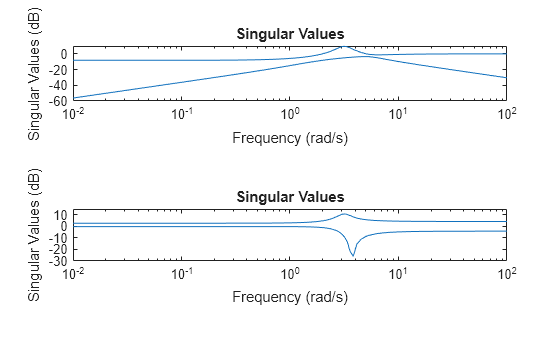
Consider the following two-input, two-output dynamic system.
Compute the singular value responses of H(s) and I + H(s).
H = [0, tf([3 0],[1 1 10]) ; tf([1 1],[1 5]), tf(2,[1 6])];
[svH,wH] = sigma(H);
[svIH,wIH] = sigma(H,[],2);
In the last command, the input 2 selects the second response type, I + H(s). The vectors svH and svIH contain the singular value response data, at the frequencies in wH and wIH.
Plot the singular value responses of both systems.
subplot(211)
sigma(H)
subplot(212)
sigma(H,[],2)
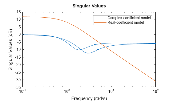
Create a singular value plot of a model with complex coefficients and a model with real coefficients on the same plot.
rng(0)
A = [-3.50,-1.25-0.25i;2,0];
B = [1;0];
C = [-0.75-0.5i,0.625-0.125i];
D = 0.5;
Gc = ss(A,B,C,D);
Gr = rss(4);
sigma(Gc,Gr)
legend('Complex-coefficient model','Real-coefficient model');
In log frequency scale, the plot shows two branches for models with complex coefficients, one for positive frequencies, with a right-pointing arrow, and one for negative frequencies, with a left-pointing arrow. In both branches, the arrows indicate the direction of increasing frequencies. The plots for models with real coefficients always contain a single branch with no arrows.
You can change the frequency scale of the plot by right-clicking the plot and selecting Properties. In the Property Editor dialog box, on the Units tab, set the frequency scale to linear scale. Alternatively, you can use the sigmaplot function and modify the chart object properties.
Create the plot with customized options.
sp = sigmaplot(Gc,Gr);
sp.FrequencyScale = 'linear'sp =
SigmaPlot (Singular Values) with properties:
Responses: [2×1 controllib.chart.response.SigmaResponse]
Characteristics: [1×1 controllib.chart.options.CharacteristicsManager]
MagnitudeScale: "linear"
MagnitudeUnit: "dB"
FrequencyScale: "linear"
FrequencyUnit: "rad/s"
Visible: on
Show all properties
legend('Complex-coefficient model','Real-coefficient model');
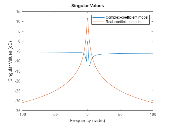
In linear frequency scale, the plot shows a single branch with a symmetric frequency range centered at a frequency value of zero. The plot also shows the negative-frequency response of a model with real coefficients when you plot the response along with a model with complex coefficients.
Input Arguments
Output Arguments
Tips
When you need additional plot customization options, use
sigmaplotinstead.Plots created using
sigmado not support multiline titles or labels specified as string arrays or cell arrays of character vectors. To specify multiline titles and labels, use a single string with anewlinecharacter.sigma(sys) title("first line" + newline + "second line");
Algorithms
sigma uses the MATLAB® function svd to compute the singular values of the complex
frequency response.
For an
frdmodel,sigmacomputes the singular values ofsys.ResponseDataat the frequencies,sys.Frequency.For continuous-time
tf,ss, orzpkmodels with transfer function H(s),sigmacomputes the singular values of H(jω) as a function of the frequency ω.For discrete-time
tf,ss, orzpkmodels with transfer function H(z) and sample time Ts,sigmacomputes the singular values offor frequencies ω between 0 and the Nyquist frequency ωN = π/Ts.