Detect Anomalies in Machinery Using LSTM Autoencoder

This example shows how to detect anomalies in vibration data from an industrial machine using a long short-term memory (LSTM) autoencoder implemented in the deepSignalAnomalyDetector object from Signal Processing Toolbox™. The example is based on Anomaly Detection in Industrial Machinery Using Three-Axis Vibration Data (Predictive Maintenance Toolbox). Refer to that example for details about the data, the feature extraction, and alternative methods of anomaly detection.

Load Data

The data for this example consists of three-channel vibration measurements from a battery electrode cutting machine, collected over several days of operation. Each channel corresponds to a vibration axis. At one point during the data collection process, the machine has a scheduled maintenance. The data collected after scheduled maintenance is assumed to represent normal operating conditions of the machine. The data from before maintenance can represent normal or anomalous conditions.

Retrieve, unzip, and load the data into the workspace.

localfile = matlab.internal.examples.downloadSupportFile("predmaint", ...
    "anomalyDetection3axisVibration/v1/vibrationData.zip");
unzip(localfile,tempdir)
data = load(fullfile(tempdir,"FeatureEntire.mat"));
features = data.featureAll;

In the Predictive Maintenance Toolbox example, you use the Diagnostic Feature Designer (Predictive Maintenance Toolbox) app to extract features from the raw data and select the features that are most effective for diagnosing faulty conditions.

• From the first channel, select the crest factor, kurtosis, root-mean-square (RMS) value, and standard deviation.

• From the second channel, select the mean, RMS value, skewness, and standard deviation.

• From the third channel, select the crest factor, signal to noise and distortion ratio (SINAD), signal-to-noise ratio (SNR), and total harmonic distortion (THD).

In this example, you represent each signal by its associated set of 12 features. The data file labels each signal as being extracted from data measured before or after the maintenance. Shorten the variable names by removing the redundant phrase "_stats/Col1_". Display a few random rows of the table.

for ik = 2:size(features,2)
    features.Properties.VariableNames(ik) = ...
        erase(features.Properties.VariableNames(ik),"_stats/Col1_");
end
head(features(randperm(height(features)),:))

    label     ch1CrestFactor    ch1Kurtosis    ch1RMS    ch1Std     ch2Mean      ch2RMS     ch2Skewness    ch2Std     ch3CrestFactor    ch3SINAD    ch3SNR     ch3THD 
    ______    ______________    ___________    ______    ______    __________    _______    ___________    _______    ______________    ________    _______    _______

    After         1.6853          1.7668       3.1232    3.1229     0.0033337    0.49073      1.5804       0.49073        9.8948        -9.2412     -9.0909    -5.4062
    After         1.9119          2.2294        2.753    2.7525    -0.0097274    0.50029      1.7341        0.5002        6.9006        -8.0354     -7.8494    -5.7064
    After         2.0892          2.9014       2.5194    2.5171     -0.010164    0.53292      3.9178       0.53283        6.9842        -9.0894     -8.9333    -5.4036
    After         1.7445          1.7777       3.0172    3.0161     -0.019713    0.70911      2.7898       0.70884        6.2546        -8.3171     -8.1375    -5.5683
    After         2.0058          1.7628       2.6241    2.6239     -0.039584    0.72208      5.0116         0.721        21.593        -13.534     -13.481    -5.5184
    After         1.7668          1.7662       2.9792    2.9789    -0.0034628    0.65523      2.7817       0.65522        6.8951        -8.3663     -8.1994      -5.83
    After         1.8217          2.0704       2.8893    2.8883     -0.055623    0.89943       3.615       0.89771         6.454        -7.9951     -7.8086     -5.737
    Before        2.8021          2.7288       1.8784    1.8782    -0.0020621     0.2861      2.1066       0.28609        9.0325         -15.02     -15.009    -10.604

Verify that about a third of the signals were collected before the maintenance.

countlabels(features)

ans=2×3 table
    label     Count    Percent
    ______    _____    _______

    Before     6218    35.245 
    After     11424    64.755 

Split the data into a training set containing 90% of the measurements taken at random and a test set containing the rest. Reset the random number generator for reproducible results.

rng("default")
idx = splitlabels(features,0.9,"randomized");

fTrain = features(idx{1},:);
fTest = features(idx{2},:);

Define Detector Architecture

Use the deepSignalAnomalyDetector (Signal Processing Toolbox) object to create a long short-term memory (LSTM) autoencoder. An autoencoder is a type of neural network that learns a compressed representation of unlabeled sequence data. This autoencoder differs from the one in the Predictive Maintenance Toolbox example in some details but produces similar results.

• Specify that each signal input to the detector has only one channel.

• Specify two encoder layers, one with 16 hidden units and the other with 32 hidden units, and one decoder layer with 16 hidden units.

• Specify the WindowLength property of the detector so that it treats each input signal as a single segment. Depending on the application, the detector can also be trained to detect anomalous points or regions within each signal.

• Specify that the object computes the detection threshold using the mean window loss measured over the entire training data set and multiplied by 0.8.

detector = deepSignalAnomalyDetector(1,"lstmautoencoder", ...
    EncoderHiddenUnits=[16 32], ...
    DecoderHiddenUnits=16, ...
    WindowLength="fullSignal", ...
    ThresholdMethod="mean", ...
    ThresholdParameter=0.8);

Prepare Data for Training

Define a function to convert the data to a format suitable for input to the anomaly detector. The function removes the categorical column from the data matrix, converts the numeric matrix to a cell array in which each cell represents a matrix row, and transposes each cell.

t2c = @(in)cellfun(@transpose, ...
    mat2cell(in(:,2:end).Variables,ones(height(in),1)), ...
    UniformOutput=false);

Specify Training Options

Train for 200 epochs with a mini-batch size of 500. Use the Adam solver.

options = trainingOptions("adam", ...
   Plots="training-progress", ...
   Verbose=false, ...
   MiniBatchSize=500,...
   MaxEpochs=200);

Train Detector

Use the trainDetector (Signal Processing Toolbox) function to train the LSTM autoencoder with unlabeled data assumed to be normal. This is an example of unsupervised training.

trainAfter = fTrain(fTrain.label=="After",:);

trainDetector(detector,t2c(trainAfter),options)

Test Detector

When you give the trained autoencoder a testing data set, the object reconstructs each signal based on what it learned during the training. The object then computes a reconstruction loss that measures the deviation between the signal and its reconstruction and identifies a signal as anomalous when the reconstruction error exceeds the specified threshold. The detect (Signal Processing Toolbox) function outputs a logical array that is true for anomalous signals.

Count the anomalies in the testing data collected before the scheduled maintenance. Express the number of anomalies as a percentage of the number of signals.

testBefore = fTest(fTest.label=="Before",:);

aBefore = cell2mat(detect(detector,t2c(testBefore)));
nBefore = sum(aBefore)/height(testBefore)*100

nBefore = 99.0354

Count the anomalies in the testing data collected after the scheduled maintenance. Express the number of anomalies as a percentage of the number of signals and verify that the value is much smaller than for the pre-maintenance data.

testAfter = fTest(fTest.label=="After",:);

aAfter = cell2mat(detect(detector,t2c(testAfter)));
nAfter = sum(aAfter)/height(testAfter)*100

nAfter = 2.9772

Visualize and characterize randomly chosen sample signals corresponding to normal and abnormal conditions. The plotAnomalies (Signal Processing Toolbox) function displays the input signal and its reconstruction by the autoencoder. The second output argument of the detect function is the aggregated reconstruction loss for each input signal.

[~,lB] = detect(detector,t2c(testBefore));

ndN = find(~aBefore);
ndN = ndN(randi(length(ndN)));
plotAnomalies(detector,t2c(testBefore(ndN,:)), ...
    PlotReconstruction=true)
text(2,-3,"Signal " + ndN + ", Loss = " + lB(ndN))
ylim([-16 11])
grid on

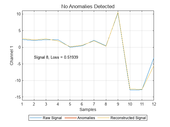
When the detector identifies a signal as anomalous, it shows that signal with a thicker line and in a different color.

ndA = find(aBefore);
ndA = ndA(randi(length(ndA)));
plotAnomalies(detector,t2c(testBefore(ndA,:)), ...
    PlotReconstruction=true)
text(2,-3,"Signal " + ndA + ", Loss = " + lB(ndA))
ylim([-16 11])
grid on

Plot Loss and Vizualize Threshold

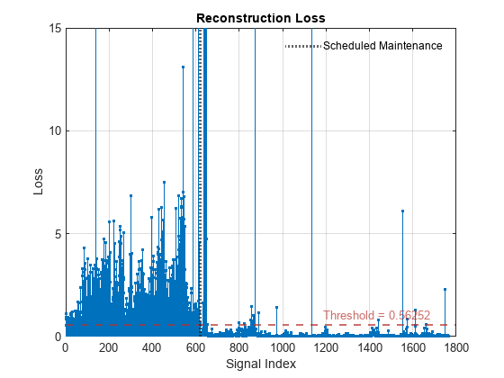
Use the plotLoss (Signal Processing Toolbox) function to plot the signal-by-signal reconstruction loss for the testing data before and after the scheduled maintenance. As expected, the reconstruction losses for the pre-maintenance data are much higher than for the post-maintenance data. The function also displays the computed threshold.

clf
q = plotLoss(detector,t2c(fTest));
xl = xline(height(testBefore),":",LineWidth=2, ...
    DisplayName="Scheduled Maintenance");
legend(xl,Box="off")
ylim([0 15])

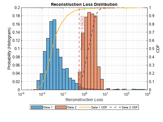
The plotLossDistribution (Signal Processing Toolbox) function displays the cumulative distribution function (CDF) and a histogram of the reconstruction losses that the detector computes. Compare the reconstruction loss distribution for the post-maintenance testing data and the pre-maintenance data. You can adjust the threshold to provide better separation between the normal data and the anomalous data.

plotLossDistribution(detector,t2c(testAfter),t2c(testBefore))

The receiver operating characteristic (ROC) curve for a detector or classifier describes its performance as the separation threshold varies. The area under the ROC curve (AUC) summarizes the information given by the curve. An AUC value close to 1 indicates that the detector or classifier performs well. Plot the ROC curve and compute the AOC for the anomaly detector in this example.

[~,lT] = detect(detector,t2c(fTest));
rocc = rocmetrics(fTest.label=="Before",cell2mat(lT),true);
plot(rocc,ShowModelOperatingPoint=false)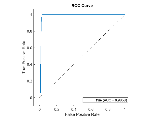

Conclusion

This example introduces the deepSignalAnomalyDetector object and uses it to detect anomalies in vibration data from an industrial machine.