dsp.DynamicFilterVisualizer
Display time-varying magnitude and phase response of digital filters
Description
The dsp.DynamicFilterVisualizer object displays the magnitude
response and phase response of time-varying digital filters or time-varying filter
coefficients. The input to this object can be a filter coefficients vector or a filter
System object™.
Using the dynamic filter visualizer, you can configure the plot settings, find the peak values, enable cursor measurements, and even generate script to recreate the plot with the current settings from the visualizer interface. For details, see Configure Filter Visualizer.
Creation
Syntax
Description
dfv = dsp.DynamicFilterVisualizerdfv, that displays the magnitude
response of digital filters or filter coefficients.
dfv = dsp.DynamicFilterVisualizer(nfft)NumFrequencyPoints
property set to nfft.
dfv = dsp.DynamicFilterVisualizer(nfft,Fs)NumFrequencyPoints
property set to nfft and the SampleRate property
set to Fs.
dfv = dsp.DynamicFilterVisualizer(nfft,Fs,range)NumFrequencyPoints
property set to nfft, the SampleRate property
set to Fs, and the FrequencyRange property set
to range.
dfv = dsp.DynamicFilterVisualizer(PropertyName=Value)NumFrequencyPoints to 1024.
Properties
Frequently Used
Number of frequency points over which to compute the spectral estimate, specified as a positive integer.
Tunable: Yes
Scope Window Use
On the Scope tab, click Settings, and set Frequency Points to a positive integer.
Data Types: single | double | int8 | int16 | int32 | int64 | uint8 | uint16 | uint32 | uint64
Since R2023a
Flag to display normalized frequency, specified as one of these values:
true–– The filter visualizer displays the frequency response in normalized frequency units (0 to 1).false–– The filter visualizer displays the frequency response in Hz. You can specify the input sample rate through theSampleRateproperty.
Scope Window Use
On the Scope tab, click Settings, and select Normalized Frequency.
Data Types: logical
Sampling rate of the input signal, specified as a real positive scalar in Hz.
Tunable: Yes
Dependency
To enable this property, set
NormalizedFrequency to false. (since R2023a)
Scope Window Use
On the Scope tab, click Settings, and set Sample Rate (Hz) to a positive scalar.
Data Types: single | double | int8 | int16 | int32 | int64 | uint8 | uint16 | uint32 | uint64
Range of the frequency axis, specified as a two-element numeric vector that is monotonically increasing and of the form [fmin, fmax].
When you set the
NormalizedFrequencyproperty totrue, fmax is in normalized frequency units and must be a positive scalar that is less than or equal to 1. (since R2023a)When you set the
NormalizedFrequencyproperty tofalse, fmax is in Hz and must be less than or equal to Fs/2, where Fs is the value you specify in theSampleRateproperty. (since R2023a)
Tunable: Yes
Scope Window Use
On the Scope tab, click Settings, and set Range to a two-element numeric vector.
Data Types: single | double | int8 | int16 | int32 | int64 | uint8 | uint16 | uint32 | uint64
X-axis scale, specified as either "Linear"
or "Log".
Tunable: Yes
Scope Window Use
On the Scope tab, click Settings, and set X-Scale.
Y-axis units, specified as one of the following:
"Magnitude""Magnitude (dB)""Magnitude squared"
Tunable: Yes
Scope Window Use
On the Scope tab, click Settings, and set Display Unit.
true– The filter visualizer plots the magnitude and phase responses of the filter on two separate axes.false– The filter visualizer plots only the magnitude response of the filter.
Tunable: Yes
Scope Window Use
On the Scope tab, click the Magnitude Phase button.
Specify the type of plot to use in the filter visualizer window as one of these:
"Line"– The filter visualizer connects each point on the magnitude and phase response plot with a line."Stairs"– The filter visualizer displays the filter response (magnitude, phase, or both) as a stair-step graph. A stair-step graph is made up of only horizontal lines and vertical lines. Each horizontal line represents the filter response over a frequency value and is connected to two vertical lines. Each vertical line represents a change in values occurring at a frequency."Stem"– The filter visualizer displays the frequency response as circles with vertical lines extending down to the x-axis at each of the frequency values.
You can individually control the type of
plot for each filter response curve. To control the type of plot for each curve,
specify the PlotType property as a cell array of character
vectors or an array of strings. If you display both the magnitude and phase responses,
the visualizer applies the same plot type setting to both the response curves. (since R2025a)
Tunable: Yes
Scope Window Use
On the Scope tab, click Settings, and set Plot Type.
Specify the scaling mode for the axes as one of these:
"Auto"— The filter visualizer scales the axes as needed to fit the data, both during and after simulation."Manual"— The filter visualizer does not scale the axes automatically."OnceAtStop"— The filter visualizer scales the axes when the simulation stops."Updates"— The filter visualizer scales the axes limits once after a set number of visual updates. The number of updates is determined by the value of theAxesScalingNumUpdatesproperty.
Scope Window Use
Hover over the filter visualizer to see the maximize ![]() , pan
, pan ![]() , zoom
, zoom ![]() , and autoscale
, and autoscale ![]() buttons. You can also zoom and pan using your
mouse.
buttons. You can also zoom and pan using your
mouse.
Tunable: Yes
Data Types: char | string
Specify the number of updates before scaling as a real, positive scalar integer.
Tunable: Yes
Dependency
To enable this property, set AxesScaling to
"Updates".
Data Types: double
Measurements
Channel for which to obtain measurements, specified as a positive integer in the range [1 N], where N is the number of input channels.
Tunable: Yes
Scope Window Use
Click the Measurements tab on the Dynamic Filter Visualizer toolstrip. In the Channel section, select a Channel.
Data Types: double
Cursor measurements to display waveform cursors, specified as a CursorMeasurementsConfiguration object.
All CursorMeasurementsConfiguration properties are
tunable.
Tunable: Yes
Scope Window Use
Click the Measurements tab on the Dynamic Filter Visualizer toolstrip and modify the cursor measurements in the Cursors section.
Peak finder measurements to compute and display the largest calculated peak
values, specified as a PeakFinderConfiguration object.
All PeakFinderConfiguration
properties are tunable.
Tunable: Yes
Scope Window Use
Click the Measurements tab on the Dynamic Filter Visualizer toolstrip and modify the peak finder measurements in the Peaks section.
Visualization
Caption to display on the Dynamic Filter Visualizer window, specified as a character vector or a string scalar.
Example: "Dynamic Filter
Visualizer"
Example: "Dynamic Filter Visualizer"
Tunable: Yes
Scope window position in pixels, specified as a four-element double vector of the
form [left bottom width height]. The default value of this property is dependent on
the screen resolution, and is such that the window is positioned in the center of the
screen, with a width and height of 800 and 500
pixels, respectively.
Tunable: Yes
Data Types: single | double | int8 | int16 | int32 | int64 | uint8 | uint16 | uint32 | uint64
Specify whether to display the filter visualizer in maximized-axes mode. In this mode, the axes are expanded to fit into the entire display. To conserve space, labels do not appear in each display. Instead, tick-mark values appear on top of the plotted data. You can select one of the following options:
"Auto"— The axes appear maximized in all displays only if theTitleandYLabelproperties are empty for every display. If you enter any value in any display for either of these properties, the axes are not maximized."On"— The axes appear maximized in all displays. Any values entered into theTitleandYLabelproperties are hidden."Off"— None of the axes appear maximized.
Scope Window Use
Hover over the Dynamic Filter Visualizer window to see the maximize axes button
![]() .
.
Tunable: Yes
Data Types: char | string
Display title, specified as a character vector or a string scalar.
Example: "Magnitude Response"
Example: "Magnitude Response"
Tunable: Yes
Scope Window Use
On the Scope tab, click Settings, and set Title to a character vector or a string scalar.
Y-axis limits, specified as a two-element numeric row vector with the second element greater than the first element and of the form [ymin, ymax].
Tunable: Yes
Scope Window Use
On the Scope tab, click Settings, and set Y-Limits to a two-element numeric vector.
Data Types: single | double | int8 | int16 | int32 | int64 | uint8 | uint16 | uint32 | uint64
When this property is set to false, no legend is displayed.
When this property is set to true, a legend with automatic string
labels for each input filter is displayed.
Tunable: Yes
Scope Window Use
On the Scope tab, click Legend.
Data Types: logical
Names to label the input filters in the legend, specified as a cell array of
character vectors or an array of strings. The default is an empty cell array. When
this property is set to an empty cell array, the filters are named by default names,
such as Filter 1, Filter 2, and so on.
Tunable: Yes
Scope Window Use
On the Scope tab, click Legend. In the legend that appears on the plot, click the filter name.
Set this property to true to show grid lines on the
plot.
Scope Window Use
On the Scope tab, click Settings, and select Show Grid.
Upper limit spectral mask, specified as a two-column matrix. The first column represents the frequency values (Hz), and the second column represents the magnitude spectrum of the upper limit mask.
Tunable: Yes
Data Types: single | double | int8 | int16 | int32 | int64 | uint8 | uint16 | uint32 | uint64
Lower limit spectral mask, specified as a two-column matrix. The first column represents the frequency values (Hz), and the second column represents the magnitude spectrum of the lower limit mask.
Tunable: Yes
Data Types: single | double | int8 | int16 | int32 | int64 | uint8 | uint16 | uint32 | uint64
Color and Styling
Since R2024b
Background color in scope, specified as an RGB triplet, a hexadecimal color code, a color name, or a short name. For more information on all the acceptable values, see Color.
Tunable: Yes
Scope Window Use
On the Scope tab, click Settings, and select a Background color.
Data Types: double | char
Since R2024b
Color of the axes in the scope, specified as an RGB triplet, a hexadecimal color code, a color name, or a short name. For more information on all the acceptable values, see Color.
Tunable: Yes
Scope Window Use
On the Scope tab, click Settings, and select an Axes color.
Data Types: double | char
Since R2024b
Colors of the labels in the scope, specified as an RGB triplet, a hexadecimal color code, a color name, or a short name. Use this property to set the color of the scope title, x-axis and y-axis labels, and the axes ticks. For more information on all the acceptable values, see Color.
Tunable: Yes
Scope Window Use
On the Scope tab, click Settings, and select a Labels color.
Data Types: double | char
Since R2024b
Scope font size, specified as a positive scalar. Use this property to set the font size for the ticks, labels, title, and measurements of the scope.
Tunable: Yes
Scope Window Use
On the Scope tab, click Settings, and set the Font Size to one of the available values.
Data Types: single | double | int8 | int16 | int32 | int64 | uint8 | uint16 | uint32 | uint64
Since R2024b
Visibility of plot lines in scope, specified as one of these:
"on"or 1 –– The scope displays the plot line. If you are plotting multiple lines, the scope applies this value to all the lines."off"or 0 –– The scope hides the plot line. If you are plotting multiple lines, the scope applies this value to all the lines.vector of logical values –– The scope applies the values to the lines in the plot. The length of the vector must equal the number of lines that you are plotting in the scope.
Tunable: Yes
Scope Window Use
On the Scope tab, click Settings, and select the Visible property.
Data Types: logical
Since R2024b
Scope line style, specified as one of these options:
"-"–– Solid line"--"–– Dashed line":"–– Dotted line"-."–– Dash-dotted line"none"–– No line
If you provide a cell array or an array of these values, then the length of the array must equal the number of lines that you are plotting in the scope.
Tunable: Yes
Scope Window Use
On the Scope tab, click Settings, and set Style.
Since R2024b
Scope line width, specified as a positive scalar or a vector of positive scalar values in points, where 1 point = 1/72 of an inch. If you specify a scalar value and are plotting multiple lines, then the scope applies the same value to all the lines. If you provide a vector of values, the length of the vector must equal the number of lines that you are plotting.
If the line has markers, then the line width also affects the marker edges. The line width cannot be thinner than the width of a pixel. If you set the line width to a value that is less than the width of a pixel on your system, the line displays as one pixel wide.
Tunable: Yes
Scope Window Use
On the Scope tab, click Settings, and set Width.
Data Types: single | double | int8 | int16 | int32 | int64 | uint8 | uint16 | uint32 | uint64
Since R2024b
Scope line color, specified as a matrix of RGB triplets or an array of color names.
Matrix of RGB Triplets
Specify an m-by-3 matrix, where each row is an RGB triplet. An RGB triplet is a three-element vector containing the intensities of the red, green, and blue components of a color. The intensities must be in the range [0,1]. For example, this matrix defines the new colors as blue, dark green, and orange.
scope.LineColor = [1.0 0.0 0.0
                0.0 0.4 0.0
                1.0 0.5 0.0];
Array of Color Names or Hexadecimal Color Codes
Specify any combination of color names, short names, or hexadecimal color codes.
To specify one color, set the line color to a character vector or a string scalar. For example,
scope.LineColor =
                "red"
specifies red as the only color in the color order.To specify multiple colors, set
LineColorto a cell array of character vectors or a string array. For example,scope.LineColor = {"red","green","blue"}specifies red, green, and blue as the colors.
A hexadecimal color code starts with a hash symbol
(#) followed by three or six hexadecimal digits,
which can range from 0 to F. The
values are not case sensitive. Thus, the color codes
"#FF8800", "#ff8800",
"#F80", and "#f80" are
equivalent.
This table lists the color names and short names with the equivalent RGB triplets and hexadecimal color codes.
| Color Name | Short Name | RGB Triplet | Hexadecimal Color Code | Appearance |
|---|---|---|---|---|
"red" | "r" | [1 0 0] | "#FF0000" |
|
"green" | "g" | [0 1 0] | "#00FF00" |
|
"blue" | "b" | [0 0 1] | "#0000FF" |
|
"cyan"
| "c" | [0 1 1] | "#00FFFF" |
|
"magenta" | "m" | [1 0 1] | "#FF00FF" |
|
"yellow" | "y" | [1 1 0] | "#FFFF00" |
|
"black" | "k" | [0 0 0] | "#000000" |
|
"white" | "w" | [1 1 1] | "#FFFFFF" |
|
Scope Window Use
On the Scope tab, click Settings, and set Color.
Tunable: Yes
Data Types: single | double | char | string | cell
Since R2024b
Scope line marker symbol, specified as one of the values listed in this table. By default, the object does not display markers. Specifying a marker symbol adds markers at each data point or vertex.
Tunable: Yes
Scope Window Use
On the Scope tab, click Settings, and set Marker.
Usage
Description
dfv( displays the time-varying
magnitude response of the object filter, filt)filt, in the Dynamic Filter
Visualizer figure, as long as filt has a valid
freqz() implementation.
Input Arguments
Object Functions
Examples
Design an FIR filter with a time-varying magnitude and phase response. Plot this varying response on a dynamic filter visualizer in normalized frequency units.
Create a dsp.DynamicFilterVisualizer object. Set the PlotAsMagnitudePhase and the NormalizedFrequency properties to true.
dfv = dsp.DynamicFilterVisualizer(PlotAsMagnitudePhase=1,...
    NormalizedFrequency=true,ShowLegend=true,...
    Title="Magnitude and Phase Response",...
    FilterNames="FIR Filter")
dfv =
  dsp.DynamicFilterVisualizer handle with properties:

      NumFrequencyPoints: 2048
     NormalizedFrequency: 1
          FrequencyRange: [0 1]
                  XScale: 'Linear'
        MagnitudeDisplay: 'Magnitude (dB)'
    PlotAsMagnitudePhase: 1
             AxesScaling: 'Auto'

  Show all properties
Vary the cutoff frequency of the FIR filter k from 0.1 to 0.5 in increments of 0.001. View the varying magnitude and phase response using the dynamic filter visualizer.
for k = 0.1:0.001:0.5
    b = designLowpassFIR(FilterOrder=90,CutoffFrequency=k);
    dfv(b,1);
end

Visualize the varying magnitude response of the variable bandwidth FIR filter using the dynamic filter visualizer.
Create a dsp.DynamicFilterVisualizer object.
dfv = dsp.DynamicFilterVisualizer(YLimits=[-160 10],...
    FilterNames="Variable Bandwidth FIR Filter")
dfv =
  dsp.DynamicFilterVisualizer handle with properties:

      NumFrequencyPoints: 2048
     NormalizedFrequency: 0
              SampleRate: 44100
          FrequencyRange: [0 22050]
                  XScale: 'Linear'
        MagnitudeDisplay: 'Magnitude (dB)'
    PlotAsMagnitudePhase: 0
             AxesScaling: 'Manual'

  Show all properties
Design a bandpass variable bandwidth FIR filter with a center frequency of 5 kHz and a bandwidth of 4 kHz.
Fs = 44100;
vbw = dsp.VariableBandwidthFIRFilter(FilterType="Bandpass",...
    FilterOrder=100,...
    SampleRate=Fs,...
    CenterFrequency=5e3,...
    Bandwidth=4e3);
Vary the center frequency of the filter. Visualize the varying magnitude response of the filter using the dsp.DynamicFilterVisualizer object.
for idx  = 1:100
    dfv(vbw);
    vbw.CenterFrequency = vbw.CenterFrequency + 20;
end

Since R2024b
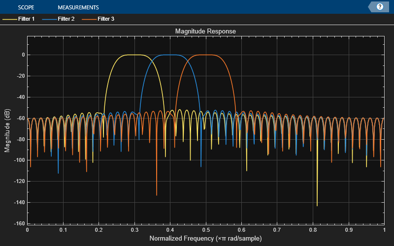
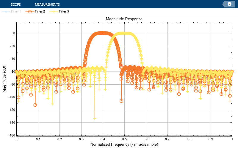
Create a dsp.DynamicFilterVisualizer object and set the NormalizedFrequency property to true. Create three bandpass FIR filters with varying center frequencies.
filtViz = dsp.DynamicFilterVisualizer(NormalizedFrequency=true);
filt1 = designBandpassFIR(FilterOrder=100,CenterFrequency=0.3,...
    Bandwidth=0.1,SystemObject=true);
filt2 = designBandpassFIR(FilterOrder=100,CenterFrequency=0.4,...
    Bandwidth=0.1,SystemObject=true);
filt3 = designBandpassFIR(FilterOrder=100,CenterFrequency=0.5,...
    Bandwidth=0.1,SystemObject=true);
Visualize the filters in the filter visualizer. This plot shows the default color and style settings of the object.
filtViz(filt1,filt2,filt3)
release(filtViz);
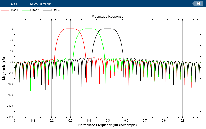
Change the background color and the axes color of the plot to "white". Set the font color to "black". Also, change the line colors to ["red" "green" "black"].
filtViz.BackgroundColor = "white";
filtViz.AxesColor = "white";
filtViz.FontColor = "black";
filtViz.LineColor = ["red" "green" "black"];
show(filtViz)
release(filtViz)
To change the color order, set LineColor to a different color order. This setting changes the color order palette.
filtViz.LineColor = colororder("glow");
show(filtViz)
release(filtViz)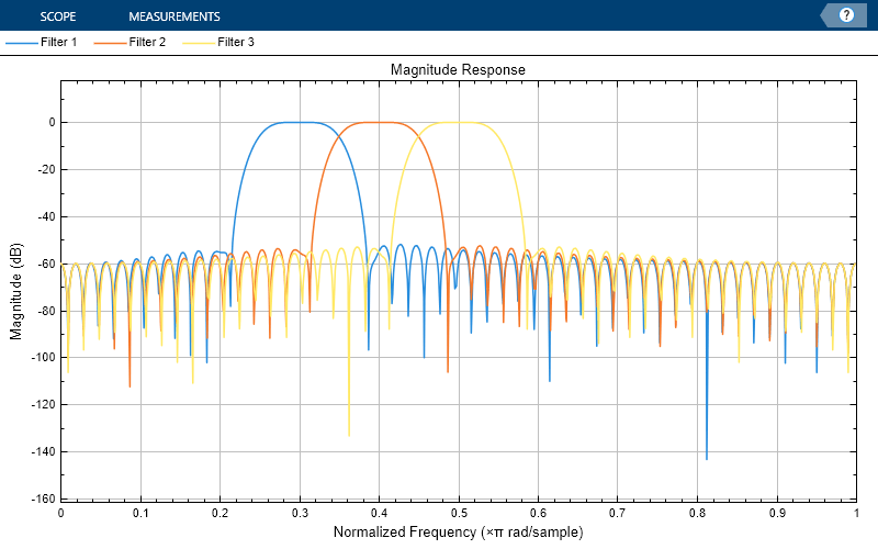
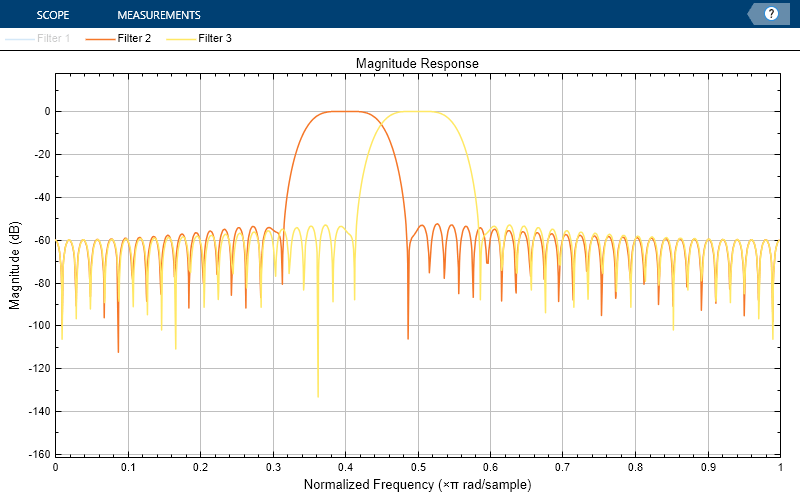
To control the visibility of the plot lines, use the LineVisible property. When you select "off", the plot line becomes invisible.
filtViz.LineVisible = ["off" "on" "on"];
show(filtViz)
release(filtViz)
You can further specify a marker for each line and change the corresponding line width.
filtViz.LineMarker = ["x","o","+"];
filtViz.LineWidth = 2;
show(filtViz)
release(filtViz)
Since R2023b
Use the printToFigure function to print the dsp.DynamicFilterVisualizer object display window to a new MATLAB® figure.
Create a dsp.DynamicFilterVisualizer object.
dfv = dsp.DynamicFilterVisualizer(YLimits=[-120 10]);
Design FIR filter with varying cutoff frequencies ranging from 0.1 to 0.5. Plot the magnitude response of the filter using the Dynamic Filter Visualizer.
for k = 0.1:0.001:0.5
    b = fir1(90, k);
    dfv(b,1);
end

Change the background color and the axes color of the plot to "white". Set the font color to "black" and the line color to "blue".
dfv.BackgroundColor = "white";
dfv.AxesColor = "white";
dfv.FontColor = "black";
dfv.LineColor = "blue";
show(dfv)
release(dfv)

Print the display of the magnitude response to a new MATLAB figure. The function returns a handle to the figure.
scopeFig = printToFigure(dfv);
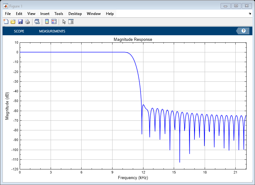
The handle to the figure scopeFig lets you modify the appearance and the behavior of the figure window.
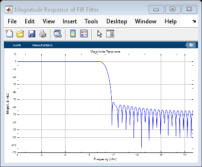
Specify a figure name and change the size of the figure to 400-by-250 pixels.
scopeFig.Name="Magnitude Response of FIR Filter";
scopeFig.NumberTitle="off";
scopeFig.Position=[1 1 400 250];
When printing to figure, you can make the figure invisible by setting the Visible argument to false.
scopeFig = printToFigure(dfv,Visible=false);
Limitations
Does not support C/C++ code generation using MATLAB® Coder™. To generate a standalone application, use the MATLAB Compiler™.
Supports MEX code generation by treating the calls to the object as extrinsic.