simplot

Plot Markov chain simulations

Syntax

simplot(mc,X)

simplot(mc,X,Name,Value)

simplot(ax,___)

h = simplot(___)

Description

simplot(mc,X) creates a heatmap from the data X on random walks through sequences of states in the discrete-time Markov chain mc.

simplot(mc,X,Name,Value) uses additional options specified by one or more name-value arguments. For example, specify the type of plot or frame rate for animated plots.

simplot(ax,___) plots on the axes specified by ax instead of the current axes (gca) using any of the input argument combinations in the previous syntaxes. The option ax can precede any of the input argument combinations in the previous syntaxes.

h = simplot(___) returns the plot handle. Use h to modify properties of the plot after you create it.

Examples

Simulate Random Walk Through Markov Chain

Consider this theoretical, right-stochastic transition matrix of a stochastic process.

$$P=\left[\begin{array}{ccccccc}0& 0& 1/2& 1/4& 1/4& 0& 0\\ 0& 0& 1/3& 0& 2/3& 0& 0\\ 0& 0& 0& 0& 0& 1/3& 2/3\\ 0& 0& 0& 0& 0& 1/2& 1/2\\ 0& 0& 0& 0& 0& 3/4& 1/4\\ 1/2& 1/2& 0& 0& 0& 0& 0\\ 1/4& 3/4& 0& 0& 0& 0& 0\end{array}\right].$$

Create the Markov chain that is characterized by the transition matrix P.

P = [ 0   0  1/2 1/4 1/4  0   0 ;
      0   0  1/3  0  2/3  0   0 ;
      0   0   0   0   0  1/3 2/3;
      0   0   0   0   0  1/2 1/2;
      0   0   0   0   0  3/4 1/4;
     1/2 1/2  0   0   0   0   0 ;
     1/4 3/4  0   0   0   0   0 ];
mc = dtmc(P);

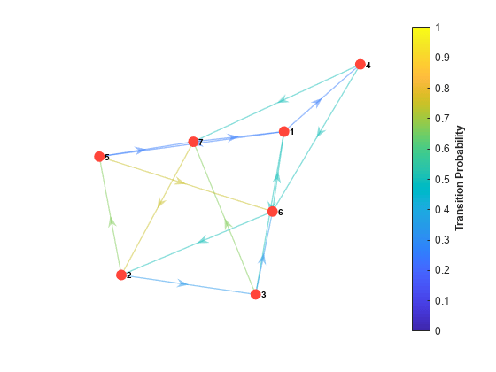
Plot a directed graph of the Markov chain. Indicate the probability of transition by using edge colors.

figure;
graphplot(mc,'ColorEdges',true);

Simulate a 20-step random walk that starts from a random state.

rng(1); % For reproducibility
numSteps = 20;
X = simulate(mc,numSteps)

X = 21×1

     3
     7
     1
     3
     6
     1
     3
     7
     2
     5
      ⋮

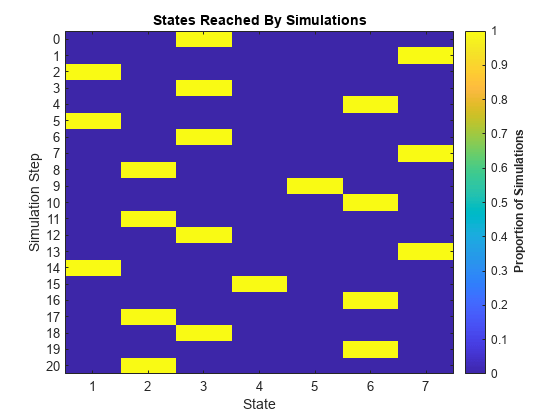
X is a 21-by-1 matrix. Rows correspond to steps in the random walk. Because X(1) is 3, the random walk begins at state 3.

Visualize the random walk.

figure;
simplot(mc,X);

Compare Theoretical and Realized Transitions

Consider this theoretical, right-stochastic transition matrix of a stochastic process.

$$P=\left[\begin{array}{ccccccc}0& 0& 1/2& 1/4& 1/4& 0& 0\\ 0& 0& 1/3& 0& 2/3& 0& 0\\ 0& 0& 0& 0& 0& 1/3& 2/3\\ 0& 0& 0& 0& 0& 1/2& 1/2\\ 0& 0& 0& 0& 0& 3/4& 1/4\\ 1/2& 1/2& 0& 0& 0& 0& 0\\ 1/4& 3/4& 0& 0& 0& 0& 0\end{array}\right].$$

Create the Markov chain that is characterized by the transition matrix P.

P = [ 0   0  1/2 1/4 1/4  0   0 ;
      0   0  1/3  0  2/3  0   0 ;
      0   0   0   0   0  1/3 2/3;
      0   0   0   0   0  1/2 1/2;
      0   0   0   0   0  3/4 1/4;
     1/2 1/2  0   0   0   0   0 ;
     1/4 3/4  0   0   0   0   0 ];
mc = dtmc(P);

Generate 100 20-step random walks starting from state 1.

rng(1); % For reproducibility
numSteps = 20;
X0 = zeros(mc.NumStates,1);
X0(1) = 100; % 100 random walks starting from state 1 only
X = simulate(mc,numSteps,'X0',X0);

X is a 21-by-100 matrix.

Visualize the proportion of times that states transition to other states for all random walks by using a heatmap.

figure;
simplot(mc,X,'Type','transitions');

Rows and columns of the heatmap correspond to state numbers.

Compare the realized transition matrix to the theoretical transition matrix by using a heatmap.

figure
imagesc(mc.P)
axis square
colorbar

The realized and theoretical transition matrices are similar.

Input Arguments

mc — Discrete-time Markov chain

dtmc object

Discrete-time Markov chain with NumStates states and transition matrix P, specified as a dtmc object. P must be fully specified (no NaN entries).

X — Simulated data

numeric matrix of positive integers

Simulated data, specified as a (1 + numSteps)-by-numSims numeric matrix of positive integers returned by simulate. The first row contains the initial states. Columns represent random walks from the corresponding initial state.

Data Types: double

ax — Axes on which to plot

Axes object

Axes on which to plot, specified as an Axes object.

By default, simplot plots to the current axes (gca).

Name-Value Arguments

Specify optional pairs of arguments as Name1=Value1,...,NameN=ValueN, where Name is the argument name and Value is the corresponding value. Name-value arguments must appear after other arguments, but the order of the pairs does not matter.

Before R2021a, use commas to separate each name and value, and enclose Name in quotes.

Example: 'Type','Graph','FrameRate',3 creates an animated plot of the simulations using a frame rate of 3 seconds.

Type — Plot type

'states' (default) | 'transitions' | 'graph'

Plot type, specified as the comma-separated pair consisting of 'Type' and a value in this table.

Value	Description
'states'	States reached by simulations in X. The plot is a (1 + numSteps)-by-NumStates heatmap. Row i displays the proportion of walks in each state at step i.
'transitions'	Transitions realized by simulations in X. The plot is a NumStates-by-NumStates heatmap. Element (i,j) displays the proportion of transitions from state i to state j in all simulations. The plot is an empirical estimate of the transition matrix mc.P.
'graph'	Animated graph of state counts (node size) and state flows (edge width) at each step. The 'FrameRate' name-value pair argument controls the animation progress.

Example: 'Type','graph'

Data Types: string | char

FrameRate — Length of discrete time steps

positive scalar

Length of discrete time steps, in seconds, for animated plots, specified as the comma-separated pair consisting of 'FrameRate' and a positive scalar.

The default is a pause at each time step. The animation proceeds when you press the space bar.

Example: 'FrameRate',3

Data Types: double

Output Arguments

h — Handle to simulation plot

graphics object

Handle to the simulation plot, returned as a graphics object. h contains a unique plot identifier, which you can use to query or modify properties of the plot.

Tips

To compare a plot of realized transitions ('Type','transitions') with the transition matrix, use:

figure
imagesc(mc.P)
axis square

Version History

Introduced in R2017b