Main Content

bvp4c

Solve boundary value problem — fourth-order method

Description

sol = bvp4c(odefun,bcfun,solinit) integrates a system of differential equations of the form y′ = f(x,y) specified by odefun, subject to the boundary conditions described by bcfun and the initial solution guess solinit. Use the bvpinit function to create the initial guess solinit, which also defines the points at which the boundary conditions in bcfun are enforced.

example

sol = bvp4c(odefun,bcfun,solinit,options) also uses the integration settings defined by options, which is an argument created using the bvpset function. For example, use the AbsTol and RelTol options to specify absolute and relative error tolerances, or the FJacobian option to provide the analytical partial derivatives of odefun.

example

Examples

collapse all

Solve a second-order BVP in MATLAB® using functions. For this example, use the second-order equation

y+y=0.

The equation is defined on the interval [0,π/2] subject to the boundary conditions

y(0)=0,

y(π/2)=2.

To solve this equation in MATLAB, you need to write a function that represents the equation as a system of first-order equations, a function for the boundary conditions, and a function for the initial guess. Then the BVP solver uses these three inputs to solve the equation.

Code Equation

Write a function that codes the equation. Use the substitutions y1=y and y2=y to rewrite the equation as a system of first-order equations.

y1=y2,

y2=-y1.

The corresponding function is

function dydx = bvpfcn(x,y)
dydx = zeros(2,1);
dydx = [y(2)
       -y(1)];
end

Note: All functions are included at the end of the example as local functions.

Code Boundary Conditions

Write a function that codes the boundary conditions in the form g(y(a),y(b))=0. In this form the boundary conditions are

y(0)=0,

y(π/2)-2=0.

The corresponding function is

function res = bcfcn(ya,yb)
res = [ya(1)
       yb(1)-2];
end

Create Initial Guess

Use the bvpinit function to create an initial guess for the solution of the equation. Since the equation relates y to y, a reasonable guess is that the solution involves trigonometric functions. Use a mesh of five points in the interval of integration. The first and last values in the mesh are where the solver applies the boundary conditions.

The function for the initial guess accepts x as an input and returns a guess for the value of y1 and y2. The function is

function g = guess(x)
g = [sin(x)
     cos(x)];
end
xmesh = linspace(0,pi/2,5);
solinit = bvpinit(xmesh, @guess);

Solve Equation

Use bvp4c with the derivative function, boundary condition function, and initial guess to solve the problem.

sol = bvp4c(@bvpfcn, @bcfcn, solinit);

Plot Solution

plot(sol.x, sol.y, '-o')

Figure contains an axes object. The axes object contains 2 objects of type line.

Local Functions

Listed here are the local functions that bvp4c uses to solve the equation.

function dydx = bvpfcn(x,y) % equation to solve
dydx = zeros(2,1);
dydx = [y(2)
       -y(1)];
end
%--------------------------------
function res = bcfcn(ya,yb) % boundary conditions
res = [ya(1)
       yb(1)-2];
end
%--------------------------------
function g = guess(x) % initial guess for y and y'
g = [sin(x)
     cos(x)];
end
%--------------------------------

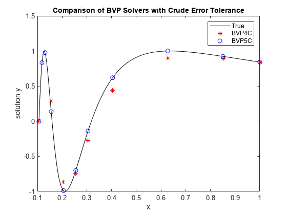
Solve a BVP at a crude error tolerance with two different solvers and compare the results.

Consider the second-order ODE

y+2xy+1x4y=0.

The equation is defined on the interval [13π,1] subject to the boundary conditions

y(13π)=0,

y(1)=sin(1).

To solve this equation in MATLAB®, you need to write a function that represents the equation as a system of first-order equations, write a function for the boundary conditions, set some option values, and create an initial guess. Then the BVP solver uses these four inputs to solve the equation.

Code Equation

With the substitutions y1=y and y2=y, you can rewrite the ODE as a system of first-order equations

y1=y2,

y2=-2xy2-1x4y1.

The corresponding function is

function dydx = bvpfcn(x,y)
dydx = [y(2)
       -2*y(2)/x - y(1)/x^4];
end

Note: All functions are included at the end of the example as local functions.

Code Boundary Conditions

The boundary condition function requires that the boundary conditions are in the form g(y(a),y(b))=0. In this form, the boundary conditions are

y(13π)=0,

y(1)-sin(1)=0.

The corresponding function is

function res = bcfcn(ya,yb)
res = [ya(1)
       yb(1)-sin(1)];
end

Set Options

Use bvpset to turn on the display of solver statistics, and specify crude error tolerances to highlight the difference in error control between the solvers. Also, for efficiency, specify the analytical Jacobian

J=fiy=[f1y1f1y2f2y1f2y2]=[01-1x4-2x].

The corresponding function that returns the value of the Jacobian is

function dfdy = jac(x,y)
dfdy = [0      1
       -1/x^4 -2/x];
end
opts = bvpset('FJacobian',@jac,'RelTol',0.1,'AbsTol',0.1,'Stats','on');

Create Initial Guess

Use bvpinit to create an initial guess of the solution. Specify a constant function as the initial guess with an initial mesh of 10 points in the interval [1/3π,1].

xmesh = linspace(1/(3*pi), 1, 10);
solinit = bvpinit(xmesh, [1; 1]);

Solve Equation

Solve the equation with both bvp4c and bvp5c.

sol4c = bvp4c(@bvpfcn, @bcfcn, solinit, opts);
The solution was obtained on a mesh of 9 points.
The maximum residual is  9.794e-02. 
There were 157 calls to the ODE function. 
There were 28 calls to the BC function. 
sol5c = bvp5c(@bvpfcn, @bcfcn, solinit, opts);
The solution was obtained on a mesh of 11 points.
The maximum error is  6.742e-02. 
There were 244 calls to the ODE function. 
There were 29 calls to the BC function. 

Plot Results

Plot the results of the two calculations for y1 with the analytic solution for comparison. The analytic solution is

y1=sin(1x),

y2=-1x2cos(1x).

xplot = linspace(1/(3*pi),1,200);
yplot = [sin(1./xplot); -cos(1./xplot)./xplot.^2];

plot(xplot,yplot(1,:),'k',sol4c.x,sol4c.y(1,:),'r*',sol5c.x,sol5c.y(1,:),'bo')
title('Comparison of BVP Solvers with Crude Error Tolerance')
legend('True','BVP4C','BVP5C')
xlabel('x')
ylabel('solution y')

Figure contains an axes object. The axes object with title Comparison of BVP Solvers with Crude Error Tolerance, xlabel x, ylabel solution y contains 3 objects of type line. One or more of the lines displays its values using only markers These objects represent True, BVP4C, BVP5C.

The plot confirms that bvp5c directly controls the true error in the calculation, while bvp4c controls it only indirectly. At more stringent error tolerances, this difference between the solvers is not as apparent.

Local Functions

Listed here are the local functions that the BVP solvers use to solve the problem.

function dydx = bvpfcn(x,y) % equation to solve
dydx = [y(2)
       -2*y(2)/x - y(1)/x^4];
end
%---------------------------------
function res = bcfcn(ya,yb) % boundary conditions
res = [ya(1)
       yb(1)-sin(1)];
end
%---------------------------------
function dfdy = jac(x,y) % analytical jacobian for f
dfdy = [0      1
       -1/x^4 -2/x];
end
%---------------------------------

Input Arguments

collapse all

Functions to solve, specified as a function handle that defines the functions to be integrated. odefun and bcfun must accept the same number of input arguments.

To code odefun, use the functional signature dydx = odefun(x,y) for a scalar x and column vector y. The return value dydx is a column vector of data type single or double that corresponds to f(x,y). odefun must accept both input arguments x and y, even if one of the arguments is not used in the function.

For example, to solve y'=5y3, use the function:

function dydx = odefun(x,y)
dydx = 5*y-3;
end

For a system of equations, the output of odefun is a vector. Each element in the vector is the solution to one equation. For example, to solve

y'1=y1+2y2y'2=3y1+2y2

use the function:

function dydx = odefun(x,y)
dydx = zeros(2,1);
dydx(1) = y(1)+2*y(2);
dydx(2) = 3*y(1)+2*y(2);
end

bvp4c also can solve problems with singularities in the solution or multipoint boundary conditions.

Example: sol = bvp4c(@odefun, @bcfun, solinit)

Unknown Parameters

If the BVP being solved includes unknown parameters, you instead can use the functional signature dydx = odefun(x,y,p), where p is a vector of parameter values. When you use this functional signature the BVP solver calculates the values of the unknown parameters starting from the initial guess for the parameter values provided in solinit.

Data Types: function_handle

Boundary conditions, specified as a function handle that computes the residual error in the boundary conditions. odefun and bcfun must accept the same number of input arguments.

To code bcfun, use the functional signature res = bcfun(ya,yb) for column vectors ya and yb. The return value res is a column vector of data type single or double that corresponds to the residual value of the boundary conditions at the boundary points.

For example, if y(a) = 1 and y(b) = 0, then the boundary condition function is

function res = bcfun(ya,yb)
res = [ya(1)-1
       yb(1)];
end
Since y(a) = 1, the residual value of ya(1)-1 should be 0 at the point x = a. Similarly, since y(b) = 0, the residual value of yb(1) should be 0 at the point x = b.

The boundary points x = a and x = b where the boundary conditions are enforced are defined in the initial guess structure solinit. For two-point boundary value problems, a = solinit.x(1) and b = solinit.x(end).

Example: sol = bvp4c(@odefun, @bcfun, solinit)

Unknown Parameters

If the BVP being solved includes unknown parameters, you instead can use the functional signature res = bcfun(ya,yb,p), where p is a vector of parameter values. When you use this functional signature the BVP solver calculates the values of the unknown parameters starting from the initial guess for the parameter values provided in solinit.

Data Types: function_handle

Initial guess of solution, specified as a structure. Use bvpinit to create solinit.

Unlike initial value problems, a boundary value problem can have no solution, a finite number of solutions, or infinitely many solutions. An important part of the process of solving a BVP is providing a guess for the required solution. The quality of this guess can be critical for the solver performance and even for a successful computation. For some guidelines on creating a good initial guess, see Initial Guess of Solution.

Example: sol = bvp4c(@odefun, @bcfun, solinit)

Data Types: struct

Option structure. Use the bvpset function to create or modify the options structure.

Example: options = bvpset('RelTol',1e-5,'Stats','on') specifies a relative error tolerance of 1e-5 and turns on the display of solver statistics.

Data Types: struct

Output Arguments

collapse all

Solution structure. You can access the fields in sol with dot-indexing, such as sol.field1. The solution (sol.x,sol.y) is continuous on the interval of integration defined in the initial mesh solinit.x and has a continuous first derivative there. You can use sol with the deval function to evaluate the solution at other points in the interval.

The structure sol has these fields.

FieldDescription

x

Mesh selected by bvp4c. This mesh typically contains different points than the initial mesh solinit.x.

y

Approximation to y(x) at the mesh points of sol.x.

yp

Approximation to y′(x) at the mesh points of sol.x.

parameters

Final values for the unknown parameters specified in solinit.parameters.

solver

'bvp4c'

stats

Computational cost statistics related to the solution: the number of mesh points, residual error, and number of calls to odefun and bcfun.

More About

collapse all

Multipoint Boundary Value Problems

For multipoint boundary value problems, the boundary conditions are enforced at several points in the interval of integration.

bvp4c can solve multipoint boundary value problems where a = a0 < a1 < a2 < ...< an = b are boundary points in the interval [a,b]. The points a1,a2,...,an−1 represent interfaces that divide [a,b] into regions. bvp4c enumerates the regions from left to right (from a to b), with indices starting from 1. In region k, [ak−1,ak], bvp4c evaluates the derivative as

yp = odefun(x,y,k) 

In the boundary conditions function bcfun(yleft,yright), yleft(:,k) is the solution at the left boundary of [ak−1,ak]. Similarly, yright(:,k) is the solution at the right boundary of region k. In particular, yleft(:,1) = y(a) and yright(:,end) = y(b).

When you create an initial guess with bvpinit, use double entries in xinit for each interface point. See the reference page for bvpinit for more information.

If yinit is a function, bvpinit calls y = yinit(x,k) to get an initial guess for the solution at x in region k. In the solution structure sol returned by bpv4c, sol.x has double entries for each interface point. The corresponding columns of sol.y contain the left and right solution at the interface, respectively.

See Solve BVP with Multiple Boundary Conditions for an example that solves a three-point boundary value problem.

Singular Boundary Value Problems

bvp4c solves a class of singular boundary value problems, including problems with unknown parameters p, of the form

y'=Syx+f(x,y,p),0=bc(y(0),y(b),p).

The interval is required to be [0, b] with b > 0. Often such problems arise when computing a smooth solution of ODEs that result from partial differential equations (PDEs) due to cylindrical or spherical symmetry. For singular problems, you specify the (constant) matrix S as the value of the 'SingularTerm' option of bvpset, and odefun evaluates only f(x,y,p). The boundary conditions and initial guess must be consistent with the necessary condition for smoothness S·y(0) = 0.

See Solve BVP with Singular Term for an example that solves a singular boundary value problem.

Algorithms

bvp4c is a finite difference code that implements the three-stage Lobatto IIIa formula [1], [2]. This is a collocation formula and the collocation polynomial provides a C1-continuous solution that is fourth-order accurate uniformly in the interval of integration. Mesh selection and error control are based on the residual of the continuous solution.

The collocation technique uses a mesh of points to divide the interval of integration into subintervals. The solver determines a numerical solution by solving a global system of algebraic equations resulting from the boundary conditions, and the collocation conditions imposed on all the subintervals. The solver then estimates the error of the numerical solution on each subinterval. If the solution does not satisfy the tolerance criteria, the solver adapts the mesh and repeats the process. You must provide the points of the initial mesh, as well as an initial approximation of the solution at the mesh points.

References

[1] Shampine, L.F., and J. Kierzenka. "A BVP Solver based on residual control and the MATLAB PSE." ACM Trans. Math. Softw. Vol. 27, Number 3, 2001, pp. 299–316.

[2] Shampine, L.F., M.W. Reichelt, and J. Kierzenka. "Solving Boundary Value Problems for Ordinary Differential Equations in MATLAB with bvp4c." MATLAB File Exchange, 2004.

Extended Capabilities

Version History

Introduced before R2006a

Go to top of page