Compare lsqnonlin and fmincon for Constrained Nonlinear Least Squares
This example shows that lsqnonlin generally takes fewer function evaluations than fmincon when solving constrained least-squares problems. Both solvers use the fmincon "interior-point" algorithm for solving the problem. Yet lsqnonlin typically solves problems in fewer function evaluations. The reason is that lsqnonlin has more information to work with. fmincon minimizes the sum of squares given as , where is a vector function. In contrast, lsqnonlin works with the entire vector , meaning it has access to all the components of the sum. In other words, fmincon can access only the value of the sum, but lsqnonlin can access each component separately.
The runlsqfmincon helper function listed at the end of this example creates a series of scaled Rosenbrock-type problems with nonlinear constraints for ranging from 1 to 50, where the number of problem variables is . For a description of the Rosenbrock function, see Solve a Constrained Nonlinear Problem, Problem-Based. The function also plots the results, showing:
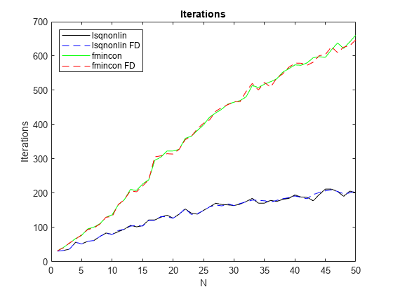
Number of iterations
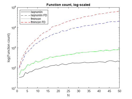
Number of function counts
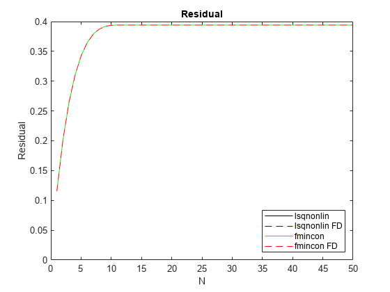
Resulting residuals
The plots show the differences between finite-difference derivative estimates (labeled FD) and derivatives calculated using automatic differentiation. For a description of automatic differentiation, see Automatic Differentiation Background.
runlsqfmincon;
The plots show the following results, which are typical.
For each , the number of iterations for
fminconis more than double that oflsqnonlinand increases approximately linearly with .The number of iterations does not depend on the derivative estimation scheme.
The function count for finite difference (FD) estimation is much higher than for automatic differentiation.
The function count for
lsqnonlinis lower than that forfminconfor the same derivative estimation scheme.The residuals match for all solution methods, meaning the results are independent of the solver and derivative estimation scheme.
The results indicate that lsqnonlin is more efficient than fmincon in terms of both iterations and function counts. However, different problems can have different results, and for some problems fmincon is more efficient than lsqnonlin.
Helper Function
This code creates the runlsqfmincon helper function.
function [lsq,lsqfd,fmin,fminfd] = runlsqfmincon()
optslsq = optimoptions("lsqnonlin",Display="none",...
    MaxFunctionEvaluations=1e5,MaxIterations=1e4); % Allow for many iterations and Fevals
optsfmincon = optimoptions("fmincon",Display="none",...
    MaxFunctionEvaluations=1e5,MaxIterations=1e4);
% Create structures to hold results
z = zeros(1,50);
lsq = struct("Iterations",z,"Fcount",z,"Residual",z);
lsqfd = lsq;
fmin = lsq;
fminfd = lsq;
rng(1) % Reproducible initial points
x00 = -1/2 + randn(50,1);
y00 = 1/2 + randn(50,1);
for N = 1:50
    x = optimvar("x",N,LowerBound=-3,UpperBound=3);
    y = optimvar("y",N,LowerBound=0,UpperBound=9);
    prob = optimproblem("Objective",sum((10*(y - x.^2)).^2 + (1 - x).^2));
    x0.x = x00(1:N);
    x0.y = y00(1:N);
    % Include a set of nonlinear inequality constraints
    cons = optimconstr(N);
    for i = 1:N
        cons(i) = x(i)^2 + y(i)^2 <= 1/2 + 1/8*i;
    end
    prob.Constraints = cons;
    [sol,fval,exitflag,output] = solve(prob,x0,Options=optslsq);
    lsq.Iterations(N) = output.iterations;
    lsq.Fcount(N) = output.funcCount;
    lsq.Residual(N) = fval;

    [sol,fval,exitflag,output] = solve(prob,x0,Options=optslsq,...
        ObjectiveDerivative="finite-differences",ConstraintDerivative="finite-differences");
    lsqfd.Iterations(N) = output.iterations;
    lsqfd.Fcount(N) = output.funcCount;
    lsqfd.Residual(N) = fval;

    [sol,fval,exitflag,output] = solve(prob,x0,Options=optsfmincon,Solver="fmincon");
    fmin.Iterations(N) = output.iterations;
    fmin.Fcount(N) = output.funcCount;
    fmin.Residual(N) = fval;

    [sol,fval,exitflag,output] = solve(prob,x0,Options=optsfmincon,Solver="fmincon",...
        ObjectiveDerivative="finite-differences",ConstraintDerivative="finite-differences");
    fminfd.Iterations(N) = output.iterations;
    fminfd.Fcount(N) = output.funcCount;
    fminfd.Residual(N) = fval;
end

N = 1:50;
plot(N,lsq.Iterations,"k",N,lsqfd.Iterations,"b--",N,fmin.Iterations,"g",N,fminfd.Iterations,"r--")
legend("lsqnonlin","lsqnonlin FD","fmincon","fmincon FD",Location="northwest")
xlabel("N")
ylabel("Iterations")
title("Iterations")

figure
semilogy(N,lsq.Fcount,"k",N,lsqfd.Fcount,"b--",N,fmin.Fcount,"g",N,fminfd.Fcount,"r--")
legend("lsqnonlin","lsqnonlin FD","fmincon","fmincon FD",Location="northwest")
xlabel("N")
ylabel("log(Function count)")
title("Function count, log-scaled")

figure
plot(N,lsq.Residual,"k",N,lsqfd.Residual,"b--",N,fmin.Residual,"g",N,fminfd.Residual,"r--")
legend("lsqnonlin","lsqnonlin FD","fmincon","fmincon FD",Location="southeast")
xlabel("N")
ylabel("Residual")
ylim([0,0.4])
title("Residual")

end