Add Safety Constraint to Simulate Two-Link Robot with SAC Agent

This example shows how to add safety constraints using control barrier functions to a Soft Actor-Critic (SAC) Agent agent trained to control a two-link robotic arm. The two-Link robot nonlinear dynamics are based on [1] and [2]. The two-link system is modeled in Simulink®.

Nonlinear Model of the Two-Link Robot

This example presents a controller design for a two link robot system. The control objective is to move the tip of the two-link robot from a starting point to a defined end point in the planar 2-D x-y space. In this example, you train a reinforcement learning agent to control the two-link robot. You then impose state-space constraints on the second-arm tip position, and simulate the deployed reinforcement learning policy using these constraints.

This figure gives the schematics of the two-link planar robot.

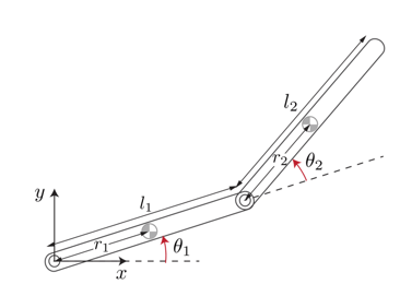
The robot configuration is described by the joint angles ${\theta }_1$, ${\theta }_2$. The robot actuators apply the torques ${\tau }_1$ and ${\tau }_2$ at the joints to control the position of the tip. The state vector is

$$\zeta \left(t\right)=\left[\begin{array}{c}{\theta }_1\\ {\theta }_2\\ {\underset{}{\overset{\dot{}}{\theta }}}_1\left(t\right)\\ {\underset{}{\overset{\dot{}}{\theta }}}_2\left(t\right)\end{array}\right]$$

The following equations describe the robot dynamics.

$$\left[\begin{array}{cc}\alpha +2\beta \cos \left(\theta {}_2\right)& \delta +\beta \cos \left(\theta {}_2\right)\\ \delta +\beta \cos \left(\theta {}_2\right)& \delta \end{array}\right]\left[\begin{array}{c}\underset{}{\overset{¨}{{\theta }_1}}\\ \underset{}{\overset{¨}{{\theta }_2}}\end{array}\right]+\left[\begin{array}{cc}-\beta \sin \left({\theta }_2\right)\underset{}{\overset{\dot{}}{{\theta }_2}}& \beta \sin \left({\theta }_2\right)\left(\underset{}{\overset{\dot{}}{{\theta }_1}}+\underset{}{\overset{\dot{}}{{\theta }_2}}\right)\\ \beta \sin \left({\theta }_2\right)\underset{}{\overset{\dot{}}{{\theta }_1}}& 0\end{array}\right]\left[\begin{array}{c}\underset{}{\overset{\dot{}}{{\theta }_1}}\\ \underset{}{\overset{\dot{}}{{\theta }_2}}\end{array}\right]=\left[\begin{array}{c}{\tau }_1\\ {\tau }_2\end{array}\right]$$

Here:

$$\alpha =I_{\text{z1}}+I_{\text{z2}}+m_1{r}_1^2+m_2\left(l_1^2+r_2^2\right)$$

$$\beta =m_2{l}_1{r}_2$$

$$\delta =I_{\text{z2}}+m_2{r}_2^2$$

Initialize the variables used by the Simulink model.

Define the physical parameters.

m1 = 3;         % Mass of link 1, kg
m2 = 2;         % Mass of link 2, kg
L1 = 0.3;       % Length of link 1, meters
L2 = 0.3;       % Length of link 2, meters

Calculate the inertia terms.

r1 = L1/2;        % Length to centroid of link 1, meters.
r2 = L2/2;        % Length to centroid of link 2, meters.
Iz1 = m1*L1^2/12; % Moment of inertia of link 1, kg*m^2
Iz2 = m2*L2^2/12; % Moment of inertia of link 2, kg*m^2

Calculate other constants.

beta = m2*L1*r2;
delta = Iz2 + m2*r2^2;
alpha = Iz1 + Iz2 + m1*r1^2 + m2*(L1^2 + r2^2);

The X-Y coordinates of the end points are functions of the link angles $\left[{\theta }_1,{\theta }_2\right]$.

Link-1:

$$\begin{array}{l}{x}_1=l_1\cos \left({\theta }_1\right)\\ y_1=l_1\sin \left({\theta }_1\right)\end{array}$$

Link-2:

$$\begin{array}{l}{x}_2={x_1+l}_2\cos \left({\theta }_1+{\theta }_2\right)\\ y_2={y_1+l}_2\sin \left({\theta }_1+{\theta }_2\right)\end{array}$$

Fix Random Number Stream for Reproducibility

The example code might involve computation of random numbers at various stages. Fixing the random number stream at the beginning of various sections in the example code preserves the random number sequence in the section every time you run it, and increases the likelihood of reproducing the results. For more information, see Results Reproducibility.

Fix the random number stream with seed 0 and random number algorithm Mersenne Twister. For more information on controlling the seed used for random number generation, see rng.

previousRngState = rng(0,"twister");

The output previousRngState is a structure that contains information about the previous state of the stream. You will restore the state at the end of the example.

Simulink Model of the Two-Link Robot with RL Agent Block

Open the model.

mdl = 'TwoLinkRobot';
open_system(mdl);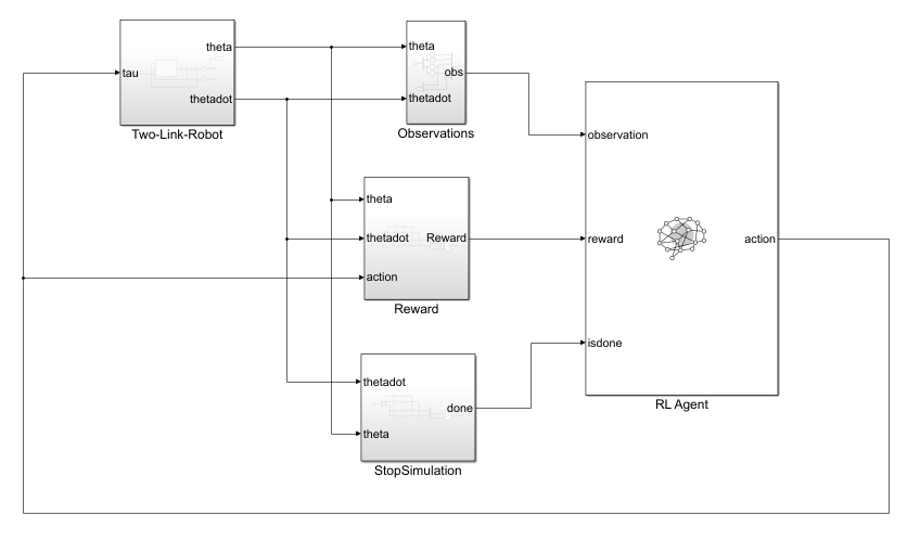

In this model:

• The initial position of the tip of the two-link robot is $\left[\begin{array}{cc}-0.5& 0\end{array}\right]$ and the final position to reach is $\left[\begin{array}{cc}0.5& 0.25\end{array}\right]$.

• The agent actions, namely, the torques for each link, are bounded between –1 to 1 N·m.

• The observation from the environment is a vector containing the cosine, sine of the link angles, and their angular rates as follows $\left[\begin{array}{cccccc}\cos \left({\theta }_1\right)& \sin \left({\theta }_1\right)& \underset{}{\overset{\dot{}}{\theta {}_1}}& \cos \left({\theta }_2\right)& \sin \left({\theta }_2\right)& \underset{}{\overset{\dot{}}{{\theta }_2}}\end{array}\right]$.

• The reward $r_t$, provided at each simulation time step, is designed as follows:

$r_t=\{\begin{array}{ll}\frac{1}{{\Vert e_t\Vert }^2}-0.001{\Vert \underset{}{\overset{\dot{}}{{\theta }_t}}\Vert }^2-0.005{\Vert u_{t-1}\Vert }^2& \text{if}{\Vert e_t\Vert }^2>0.05\\ \frac{1}{{\Vert e_t\Vert }^2}-0.001{\Vert \underset{}{\overset{\dot{}}{{\theta }_t}}\Vert }^2-0.005{\Vert u_{t-1}\Vert }^2+100& {\text{if}\Vert e_t\Vert }^2\le 0.05\end{array}$

where

• $e_t$ is the position error of the tip of the two-link arms $e_t=X^{*}-X\left(t\right)$ and $X=\left[x_2\left(t\right),y_2\left(t\right)\right]$ and $X^{*}=\left[x_2^{*},y_2^{*}\right]$.

• $\underset{}{\overset{\dot{}}{{\theta }_t}}$ is the vector containing the angular rate the two links.

• $u_{t-1}$ is the control action from the previous time step.

Create Environment Object

Create the observation and action specifications for the environment.

The environment has a continuous state space of dimension [6,1].

ObservationInfo = rlNumericSpec([6 1]);
ObservationInfo.Name = 'Robot States';
ObservationInfo.Description = 'theta1,dtheta1,theta2,dtheta2';

The environment has a continuous action space of dimension [2,1] corresponding to torques applied to each link by the agent. The actions are bounded in the [-1, 1] range.

% Initialize Action settings
ActionInfo = rlNumericSpec([2 1]);
ActionInfo.LowerLimit = -1;
ActionInfo.UpperLimit =  1;
ActionInfo.Name = 'Link Torques';

Create the environment object.

env = rlSimulinkEnv("TwoLinkRobot","TwoLinkRobot/RL Agent",...
    ObservationInfo,ActionInfo);

Specify the agent sample time Ts and the simulation time Tf in seconds.

Ts = 0.01;
Tf = 5;

Create Soft Actor Critic Agent

When you create the agent, the actor and critic networks are initialized randomly. Ensure reproducibility of the section by fixing the seed used for random number generation.

rng(0,"twister")

Create the agent options object.

agentOpts = rlSACAgentOptions;

To ensure that the RL Agent block in the environment executes every Ts seconds instead of the default setting of 1 second, set the SampleTime property of the agent.

agentOpts.SampleTime = Ts;

Set a lower learning rate to promote a smoother (though possibly slower) training.

agentOpts.ActorOptimizerOptions = rlOptimizerOptions(LearnRate= 1e-3);
agentOpts.CriticOptimizerOptions = rlOptimizerOptions(LearnRate= 1e-3);

Create a default rlSACAgent object using the environment specification and agent options object.

agent = rlSACAgent(ObservationInfo, ActionInfo,agentOpts);

Train SAC Agent

To train the agent, first specify the training options. For this example, use the following options.

• Run training for a maximum of 5000 episodes, with each episode lasting at most ceil(Tf/Ts) time steps.

• Display the training progress in the Reinforcement Learning Training Monitor dialog box (set the Plots option) and disable the command line display (set the Verbose option to false).

• Stop training when the agent receives an average cumulative reward greater than 6e4. At this point, the agent is able to reach its goal using minimal control effort.

• Save a copy of the agent for each episode where the cumulative reward is greater than 6e4.

For more information on training options, see rlTrainingOptions.

maxepisodes = 5000;
maxsteps = ceil(Tf/Ts);
trainOpts = rlTrainingOptions(...
    MaxEpisodes=maxepisodes, ...
    MaxStepsPerEpisode=maxsteps, ...
    ScoreAveragingWindowLength=5, ...
    Verbose=false, ...
    Plots="training-progress",...
    StopTrainingCriteria="AverageReward", ...
    StopTrainingValue=6e4, ...
    SaveAgentCriteria="AverageReward", ...
    SaveAgentValue=6e4);

Train the agent using the train function. Training an agent is a computationally intensive process and can take a long time. To save time while running this example, load a pretrained agent by setting doTraining to false. To train the agent yourself, set doTraining to true.

doTraining = false;
if doTraining
    % Train the agent.
    trainingResults = train(agent,env,trainOpts);
else
    % Load the pretrained agent for the example.
    load("TwoLinkRobotSAC.mat","agent")
end

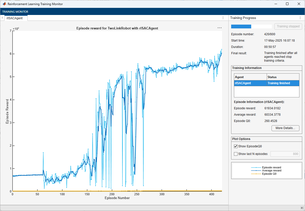
The training completes successfully after 420 episodes.

Simulate SAC Agent

For reproducibility, fix the seed for random number generation.

rng(0,"twister");

To validate the performance of the trained agent, simulate the two-link robot using the trained policy.

out = sim(mdl);

Animate the two-link robot. The helper function PlotTwoLinkArm plots the robot configuration.

theta = squeeze(out.simout.Data);
blockVisible = false;

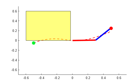
In the following plot, the green and red circles represent the initial and desired final position of the tip, respectively, while the dashed line represents the tip trajectory.

PlotTwoLinkArm(theta,0.5,0.25,L1,L2,blockVisible)

The figure shows that the agent successfully moves the robot so that the tip reaches the desired position.

Constrain Environment

The baseline SAC policy is trained in an unconstrained environment. However, here you add an obstacle in the workspace of the two-link robot. In the following picture, the yellow square represents the obstacle. As you can see, the baseline policy is not safe and the arm tip collides with the obstacle.

blockVisible = true;
PlotTwoLinkArm(theta,0.5,0.25,L1,L2,blockVisible)

To solve this problem you need to impose a safety constraint so that the tip of second link stays clear of the obstacle while going from the start to the end position.

This can be done in two ways:

1. Modify the environment to provide a large penalty upon constraint violation and/or add a constraint enforcement. Then train a new agent within the new environment. This approach could produce a near-optimal policy, but it requires you to modify the environment, and retrain the agent which is computationally expensive. Furthermore, with stochastic agents, there is always a non zero probability that constraints can be violated even with a trained policy. Finally, it is hard to train an agent for changing constraints.

2. Add an external safety constraints like an high-order control barrier function (CBF) over the policy trained within the unconstrained environment. This approach is not general as requires plant information and it only applies to control-affine plants. Furthermore, it often results in a sub-optimal solution. However, it does not allow for constraint violation, it is computationally inexpensive, and can be easily modified for different or changing constraints.

In this example you use the second approach.

Simulink Model of the Two-Link Robot with RL Agent and CBF Subsystem

The Simulink model TwoLinkRobot_HOCBF_SAC contains the RL Agent block, the Two-Link robot dynamics, and the high-order CBF subsystem.

mdl = 'TwoLinkRobot_HOCBF_SAC';
open_system(mdl);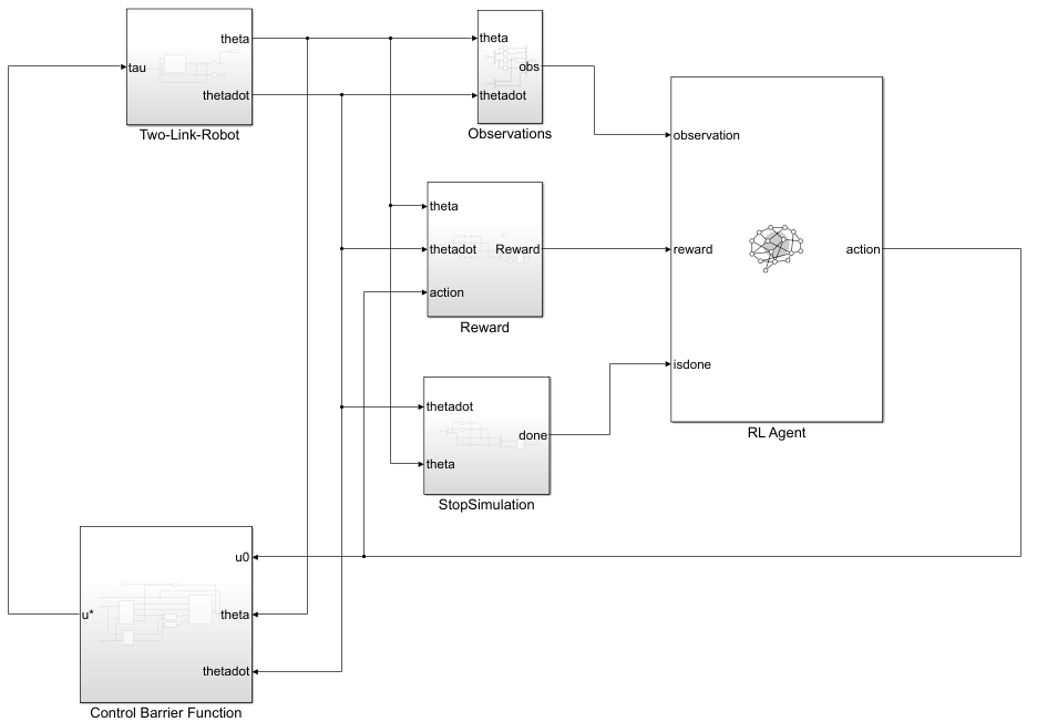

To view the CBF implementation, open the Control Barrier Function subsystem. Here, two MATLAB Function (Simulink) blocks calculate the barrier function and the several derivatives, while the High-Order Control Barrier Function (Simulink Control Design) block enforces the constraint on the control action.

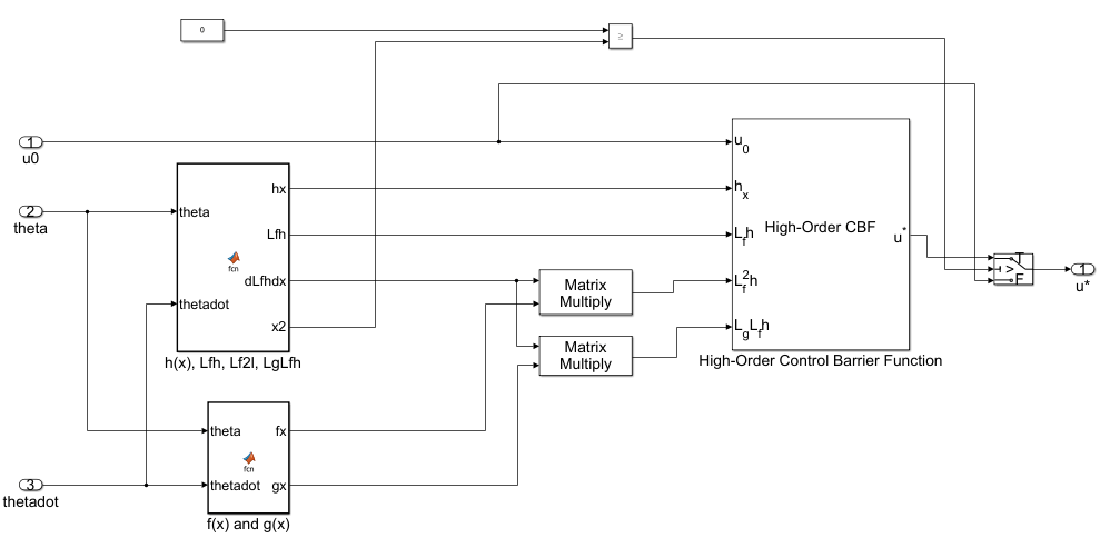
The algorithm behind the implementation of the Control Barrier Function subsystem is explained in the Algorithm: Guarantee Safety of Two-Link Robot using Control Barrier Function section at the end of the example.

Simulate Closed Loop System with High-Order CBF Constraint

For reproducibility, fix the seed of the random number generator.

rng(0,"twister");

To validate the performance of the trained agent with safety constraints, use sim (Simulink) to simulate the trained agent in the loop with the two-link robot and the control barrier function.

out = sim(mdl);

Show the robot trajectory.

theta = squeeze(out.simout.Data);
blockVisible = true;
PlotTwoLinkArm(theta,0.5,0.25,L1,L2,blockVisible)

The High-Order CBF block successfully constrains the tip of the two-link robot to avoid the obstacle.

Restore the random number stream using the information stored in previousRngState.

rng(previousRngState);

Algorithm: Guarantee Safety of Two-Link Robot using Control Barrier Function

A control barrier function (CBF) can guarantee that the state of a system remains within a specified safe region.Therefore, you can use a CBF to guarantee the safety of a controlled system.

The CBF works by imposing constraints on the control input at each time step, thereby preventing the system from entering an unsafe region [3]. Specifically, at each time step, the algorithm solves a quadratic program to constrain the control input so that the derivative of the barrier function along the system trajectory does not fall below a given threshold. For more information, see Enforce Safety Constraints with Control Barrier Functions (Simulink Control Design).

For the problem in this example, the tip of second link must not hit the obstacle.

You can mathematically model this safety constraint as the following control barrier function:

$$h\left(x\right)=\{\begin{array}{ll}-y_2\left(t\right)& x_2\left(t\right)\le 0\\ \text{no}\text{constraint}& x_2\left(t\right)>0\end{array}$$

Using the Cartesian coordinates of the end point of second link, the CBF can be written as:

$$h\left(\zeta \right)=-{l_1\sin \left({\theta }_1\right)-l}_2\sin \left({\theta }_1+{\theta }_2\right)$$

where $\zeta =\left[\begin{array}{cc}{\theta }_1& {\theta }_2\end{array}\right]$

Using the control barrier function theory described in Enforce Safety Constraints with Control Barrier Functions (Simulink Control Design), you can write the constraint equation for safe control as:

$$\underset{}{\overset{\dot{}}{h}}\left(\zeta ,u\right)\ge -\gamma h\left(\zeta \right)$$

Taking the first Lie derivative of the barrier function with respect to the states of the two-link robot yields:

$$\begin{array}{l}\underset{}{\overset{\dot{}}{h}}\left(\zeta ,u\right)=\frac{\partial h}{\partial \zeta }\underset{}{\overset{\dot{}}{\zeta }}\\ \underset{}{\overset{\dot{}}{h}}\left(\zeta ,u\right)=-\left[\begin{array}{cc}{l_1\cos \left({\theta }_1\right)+l}_2\cos \left({\theta }_1+{\theta }_2\right)& l_2\cos \left({\theta }_1+{\theta }_2\right)\end{array}\right]\left[\begin{array}{c}\underset{}{\overset{\dot{}}{{\theta }_1}}\\ \underset{}{\overset{\dot{}}{{\theta }_2}}\end{array}\right]\end{array}$$

Because the control term $u\left(t\right)$ does not appear in the first Lie derivative, take the second Lie derivative with respect to$\left[\underset{}{\overset{\dot{}}{{\theta }_1}},\underset{}{\overset{\dot{}}{{\theta }_2}}\right]$:

$$\begin{array}{l}\underset{}{\overset{¨}{h}}\left(\zeta ,u\right)=\frac{\partial h}{\partial \underset{}{\overset{\dot{}}{{\theta }_1}}}\underset{}{\overset{\dot{}}{{\theta }_1}}+\frac{\partial h}{\partial \underset{}{\overset{\dot{}}{{\theta }_2}}}\underset{}{\overset{\dot{}}{{\theta }_2}}\\ \underset{}{\overset{¨}{h}}\left(\zeta ,u\right)=-\left[\begin{array}{cc}{l_1\cos \left({\theta }_1\right)+l}_2\cos \left({\theta }_1+{\theta }_2\right)& l_2\cos \left({\theta }_1+{\theta }_2\right)\end{array}\right]\left[\begin{array}{c}\underset{}{\overset{¨}{{\theta }_1}}\\ \underset{}{\overset{¨}{{\theta }_2}}\end{array}\right]\end{array}$$

The second Lie derivative involves the term $\left[\underset{}{\overset{¨}{{\theta }_1}},\underset{}{\overset{¨}{{\theta }_2}}\right]$. Hence the control term appears through system dynamics as follows:

$\underset{}{\overset{¨}{h}}\left(\zeta ,u\right)=L_f^{2}h+L_g{L}_{f}hu=-\left[\begin{array}{cc}{l_1\cos \left({\theta }_1\right)+l}_2\cos \left({\theta }_1+{\theta }_2\right)& l_2\cos \left({\theta }_1+{\theta }_2\right)\end{array}\right]f\left(\zeta \right)-\left[\begin{array}{cc}{l_1\cos \left({\theta }_1\right)+l}_2\cos \left({\theta }_1+{\theta }_2\right)& l_2\cos \left({\theta }_1+{\theta }_2\right)\end{array}\right]g\left(\zeta \right)u$

where $L_f^{2}h=-\left[\begin{array}{cc}{l_1\cos \left({\theta }_1\right)+l}_2\cos \left({\theta }_1+{\theta }_2\right)& l_2\cos \left({\theta }_1+{\theta }_2\right)\end{array}\right]f\left(\zeta \right)$ and $L_g{L}_{f}h=-\left[\begin{array}{cc}{l_1\cos \left({\theta }_1\right)+l}_2\cos \left({\theta }_1+{\theta }_2\right)& l_2\cos \left({\theta }_1+{\theta }_2\right)\end{array}\right]g\left(\zeta \right)$

and the plant model equations $f\left(\zeta \right)$and $g\left(\zeta \right)$ are:

$f\left(\zeta \right)={\left[\begin{array}{cc}\alpha +2\beta \cos \left(\theta {}_2\right)& \delta +\beta \cos \left(\theta {}_2\right)\\ \delta +\beta \cos \left(\theta {}_2\right)& \delta \end{array}\right]}^{-1}\left[\begin{array}{cc}-\beta \sin \left({\theta }_2\right)\underset{}{\overset{\dot{}}{{\theta }_2}}& \beta \sin \left({\theta }_2\right)\left(\underset{}{\overset{\dot{}}{{\theta }_1}}+\underset{}{\overset{\dot{}}{{\theta }_2}}\right)\\ \beta \sin \left({\theta }_2\right)\underset{}{\overset{\dot{}}{{\theta }_1}}& 0\end{array}\right]\left[\begin{array}{c}\underset{}{\overset{\dot{}}{{\theta }_1}}\\ \underset{}{\overset{\dot{}}{{\theta }_2}}\end{array}\right]$ , $g\left(\zeta \right)={\left[\begin{array}{cc}\alpha +2\beta \cos \left(\theta {}_2\right)& \delta +\beta \cos \left(\theta {}_2\right)\\ \delta +\beta \cos \left(\theta {}_2\right)& \delta \end{array}\right]}^{-1}$ and $u=\left[\begin{array}{c}{\tau }_1\\ {\tau }_2\end{array}\right]$

You can then write the QP problem formulation for the two-link robot as follows:

$$\begin{array}{l}{u}^{*}=\underset{u}{\min }\frac{1}{2}{\Vert u-u_{\text{pid}}\Vert }^2\\ s.t{L}_f^{2}h+L_g{L}_{f}hu+{\gamma }_{1}h+{\gamma }_2{L}_{f}h\ge 0\end{array}$$

And implement it using the High-Order Control Barrier Function (Simulink Control Design) block as done in the Control Barrier Function subsystem in the TwoLinkRobot_HOCBF_SAC model.

References

[1] Murray, Richard M., Zexiang Li, and Shankar Sastry. A Mathematical Introduction to Robotic Manipulation. Boca Raton: CRC Press, 1994.

[2] Seiler, Peter, Robert M. Moore, Chris Meissen, Murat Arcak, and Andrew Packard. “Finite Horizon Robustness Analysis of LTV Systems Using Integral Quadratic Constraints.” Automatica 100 (February 2019): 135–43. https://doi.org/10.1016/j.automatica.2018.11.009.

[3] W. Xiao and C. Belta, "High-Order Control Barrier Functions," in IEEE Transactions on Automatic Control, vol. 67, no. 7, pp. 3655-3662, July 2022, doi: 10.1109/TAC.2021.3105491. https://doi.org/10.1109/TAC.2006.882372.