dtw

Distance between signals using dynamic time warping

Syntax

dist = dtw(x,y)

[dist,ix,iy] = dtw(x,y)

[___] = dtw(x,y,maxsamp)

[___] = dtw(___,metric)

dtw(___)

Description

dist = dtw(x,y) stretches two vectors, x and y, onto a common set of instants such that dist, the sum of the Euclidean distances between corresponding points, is smallest. To stretch the inputs, dtw repeats each element of x and y as many times as necessary. If x and y are matrices, then dist stretches them by repeating their columns. In that case, x and y must have the same number of rows.

[dist,ix,iy] = dtw(x,y) returns the common set of instants, or warping path, such that x(ix) and y(iy) have the smallest possible dist between them.

The vectors ix and iy have the same length. Each contains a monotonically increasing sequence in which the indices to the elements of the corresponding signal, x or y, are repeated the necessary number of times.

When x and y are matrices, ix and iy are such that x(:,ix) and y(:,iy) are minimally separated.

[___] = dtw(x,y,maxsamp) restricts the warping path to be within maxsamp samples of a straight-line fit between x and y. This syntax returns any of the output arguments of previous syntaxes.

[___] = dtw(___,metric) specifies the distance metric to use in addition to any of the input arguments in previous syntaxes.

dtw(___) without output arguments plots the original and aligned signals.

• If the signals are real vectors, the function displays the two original signals on a subplot and the aligned signals in a subplot below the first one.

• If the signals are complex vectors, the function displays the original and aligned signals in three-dimensional plots.

• If the signals are real matrices, the function uses imagesc to display the original and aligned signals.

• If the signals are complex matrices, the function plots their real and imaginary parts in the top and bottom half of each image.

Examples

Dynamic Time Warping of Chirp and Sinusoid

Generate two real signals: a chirp and a sinusoid.

x = cos(2*pi*(3*(1:1000)/1000).^2);
y = cos(2*pi*9*(1:399)/400);

Use dynamic time warping to align the signals such that the sum of the Euclidean distances between their points is smallest. Display the aligned signals and the distance.

dtw(x,y);

Change the sinusoid frequency to twice its initial value. Repeat the computation.

y = cos(2*pi*18*(1:399)/400);

dtw(x,y);

Add an imaginary part to each signal. Restore the initial sinusoid frequency. Use dynamic time warping to align the signals by minimizing the sum of squared Euclidean distances.

x = exp(2i*pi*(3*(1:1000)/1000).^2);
y = exp(2i*pi*9*(1:399)/400);

dtw(x,y,'squared');

Align Writing Samples

Devise a typeface that resembles the output of early computers. Use it to write the word MATLAB®.

chr = @(x)dec2bin(x')-48;

M = chr([34 34 54 42 34 34 34]);
A = chr([08 20 34 34 62 34 34]);
T = chr([62 08 08 08 08 08 08]);
L = chr([32 32 32 32 32 32 62]);
B = chr([60 34 34 60 34 34 60]);

MATLAB = [M A T L A B];

Corrupt the word by repeating random columns of the letters and varying the spacing. Show the original word and three corrupted versions. Reset the random number generator for reproducible results.

rng('default')

c = @(x)x(:,sort([1:6 randi(6,1,3)]));

subplot(4,1,1,'XLim',[0 60])
spy(MATLAB)
xlabel('')
ylabel('Original')

for kj = 2:4
    subplot(4,1,kj,'XLim',[0 60])
    spy([c(M) c(A) c(T) c(L) c(A) c(B)])
    xlabel('')
    ylabel('Corrupted')
end

Generate two more corrupted versions of the word. Align them using dynamic time warping.

one = [c(M) c(A) c(T) c(L) c(A) c(B)];
two = [c(M) c(A) c(T) c(L) c(A) c(B)];

[ds,ix,iy] = dtw(one,two);

onewarp = one(:,ix);
twowarp = two(:,iy);

Display the unaligned and aligned words.

figure

subplot(4,1,1)
spy(one)
xlabel('')
ylabel('one')

subplot(4,1,2)
spy(two,'r')
xlabel('')
ylabel('two')

subplot(4,1,3)
spy(onewarp)
xlabel('')
ylabel('onewarp')

subplot(4,1,4)
spy(twowarp,'r')
xlabel('')
ylabel('twowarp')

Repeat the computation using the built-in functionality of dtw.

dtw(one,two);

Constrained Warping Path

Generate two signals consisting of two distinct peaks separated by valleys of different lengths. Plot the signals.

x1 = [0 1 0 0 0 0 0 0 0 0 0 1 0]*.95;
x2 = [0 1 0 1 0]*.95;

subplot(2,1,1)
plot(x1)
xl = xlim;
subplot(2,1,2)
plot(x2)
xlim(xl)

Align the signals with no restriction on the warping path. To produce perfect alignment, the function needs to repeat only one sample of the shorter signal.

figure
dtw(x1,x2);

Plot the warping path and the straight-line fit between the two signals. To achieve alignment, the function expands the trough between the peaks generously.

[d,i1,i2] = dtw(x1,x2);

figure
plot(i1,i2,'o-',[i1(1) i1(end)],[i2(1) i2(end)])

Repeat the computation, but now constrain the warping path to deviate at most three elements from the straight-line fit. Plot the stretched signals and the warping path.

[dc,i1c,i2c] = dtw(x1,x2,3);

subplot(2,1,1)
plot([x1(i1c);x2(i2c)]','.-')
title(['Distance: ' num2str(dc)])
subplot(2,1,2)
plot(i1c,i2c,'o-',[i1(1) i1(end)],[i2(1) i2(end)])

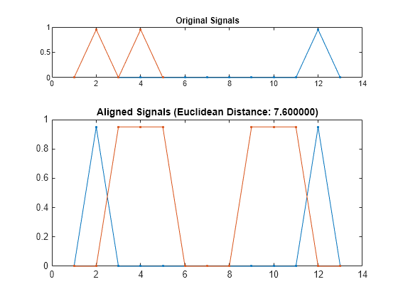
The constraint precludes the warping from concentrating too much on a small subset of samples, at the expense of alignment quality. Repeat the calculation with a one-sample constraint.

dtw(x1,x2,1);

Dynamic Time Warping of Speech Signals

Load a speech signal sampled at $$F_s=7418Hz$$. The file contains a recording of a female voice saying the word "MATLAB®."

load mtlb

% To hear, type soundsc(mtlb,Fs)

Extract the two segments that correspond to the two instances of the /æ/ phoneme. The first one occurs roughly between 150 ms and 250 ms, and the second one between 370 ms and 450 ms. Plot the two waveforms.

a1 = mtlb(round(0.15*Fs):round(0.25*Fs));
a2 = mtlb(round(0.37*Fs):round(0.45*Fs));

subplot(2,1,1)
plot((0:numel(a1)-1)/Fs+0.15,a1)
title('a_1')
subplot(2,1,2)
plot((0:numel(a2)-1)/Fs+0.37,a2)
title('a_2')
xlabel('Time (seconds)')

% To hear, type soundsc(a1,Fs), pause(1), soundsc(a2,Fs)

Warp the time axes so that the Euclidean distance between the signals is minimized. Compute the shared "duration" of the warped signals and plot them.

[d,i1,i2] = dtw(a1,a2);

a1w = a1(i1);
a2w = a2(i2);

t = (0:numel(i1)-1)/Fs;
duration = t(end)

duration = 
0.1297

subplot(2,1,1)
plot(t,a1w)
title('a_1, Warped')
subplot(2,1,2)
plot(t,a2w)
title('a_2, Warped')
xlabel('Time (seconds)')

% To hear, type soundsc(a1w,Fs), pause(1), sound(a2w,Fs)

Repeat the experiment with a complete word. Load a file containing the word "strong," spoken by a woman and by a man. The signals are sampled at 8 kHz.

load('strong.mat')

% To hear, type soundsc(her,fs), pause(2), soundsc(him,fs)

Warp the time axes so that the absolute distance between the signals is minimized. Plot the original and transformed signals. Compute their shared warped "duration."

dtw(her,him,'absolute');
legend('her','him')

[d,iher,ihim] = dtw(her,him,'absolute');
duration = numel(iher)/fs

duration = 
0.8394

% To hear, type soundsc(her(iher),fs), pause(2), soundsc(him(ihim),fs)

Dynamic Time Warping for Handwriting Alignment

The files MATLAB1.gif and MATLAB2.gif contain two handwritten samples of the word "MATLAB®." Load the files and align them along the x-axis using dynamic time warping.

samp1 = 'MATLAB1.gif';
samp2 = 'MATLAB2.gif';

x = double(imread(samp1));
y = double(imread(samp2));

dtw(x,y);

Input Arguments

x — Input signal

vector | matrix

Input signal, specified as a real or complex vector or matrix.

Data Types: single | double
Complex Number Support: Yes

y — Input signal

vector | matrix

Input signal, specified as a real or complex vector or matrix.

Data Types: single | double
Complex Number Support: Yes

maxsamp — Width of adjustment window

Inf (default) | positive integer

Width of adjustment window, specified as a positive integer.

Data Types: single | double

metric — Distance metric

'euclidean' (default) | 'absolute' | 'squared' | 'symmkl'

Distance metric, specified as 'euclidean', 'absolute', 'squared', or 'symmkl'. If X and Y are both K-dimensional signals, then metric prescribes d_mn(X,Y), the distance between the mth sample of X and the nth sample of Y. See Dynamic Time Warping for more information about d_mn(X,Y).

• 'euclidean' — Root sum of squared differences, also known as the Euclidean or ℓ₂ metric:

  $$d_{mn}(X,Y)=\sqrt{{\displaystyle \sum _{k=1}^K{\left(x_{k,m}-y_{k,n}\right)}^{*}\left(x_{k,m}-y_{k,n}\right)}}$$

• 'absolute' — Sum of absolute differences, also known as the Manhattan, city block, taxicab, or ℓ₁ metric:

  $$d_{mn}(X,Y)={\displaystyle \sum _{k=1}^K\left|x_{k,m}-y_{k,n}\right|}={\displaystyle \sum _{k=1}^K\sqrt{{\left(x_{k,m}-y_{k,n}\right)}^{*}\left(x_{k,m}-y_{k,n}\right)}}$$

• 'squared' — Square of the Euclidean metric, consisting of the sum of squared differences:

  $$d_{mn}(X,Y)={\displaystyle \sum _{k=1}^K{\left(x_{k,m}-y_{k,n}\right)}^{*}\left(x_{k,m}-y_{k,n}\right)}$$

• 'symmkl' — Symmetric Kullback-Leibler metric. This metric is valid only for real and positive X and Y:

  $$d_{mn}(X,Y)={\displaystyle \sum _{k=1}^K\left(x_{k,m}-y_{k,n}\right)\left(\log x_{k,m}-\log y_{k,n}\right)}$$

Output Arguments

dist — Minimum distance

positive real scalar

Minimum distance between signals, returned as a positive real scalar.

ix — Warping path for first signal

vector of indices | matrix of indices

Warping path for first signal, returned as a vector or matrix of indices.

iy — Warping path for second signal

vector of indices | matrix of indices

Warping path for second signal, returned as a vector or matrix of indices.

More About

Dynamic Time Warping

Two signals with equivalent features arranged in the same order can appear very different due to differences in the durations of their sections. Dynamic time warping distorts these durations so that the corresponding features appear at the same location on a common time axis, thus highlighting the similarities between the signals.

Consider the two K-dimensional signals

$$X=\left[\begin{array}{cccc}{x}_{1,1}& x_{1,2}& \cdots & x_{1,M}\\ x_{2,1}& x_{2,2}& \cdots & x_{2,M}\\ ⋮& ⋮& \ddots & ⋮\\ x_{K,1}& x_{K,2}& \cdots & x_{K,M}\end{array}\right]$$

and

$$Y=\left[\begin{array}{cccc}{y}_{1,1}& y_{1,2}& \cdots & y_{1,N}\\ y_{2,1}& y_{2,2}& \cdots & y_{2,N}\\ ⋮& ⋮& \ddots & ⋮\\ y_{K,1}& y_{K,2}& \cdots & y_{K,N}\end{array}\right],$$

which have M and N samples, respectively. Given d_mn(X,Y), the distance between the mth sample of X and the nth sample of Y specified in metric, dist stretches X and Y onto a common set of instants such that a global signal-to-signal distance measure is smallest.

Initially, the function arranges all possible values of d_mn(X,Y) into a lattice of the form

Then dist looks for a path through the lattice—parameterized by two sequences of the same length, ix and iy—such that

$$d={\displaystyle \sum _{\begin{array}{c}m\in \text{ix}\\ n\in \text{iy}\end{array}}{d}_{mn}(X,Y)}$$

is minimum. Acceptable dist paths start at d₁₁(X,Y), end at d_MN(X,Y), and are combinations of “chess king” moves:

• Vertical moves: (m,n) → (m + 1,n)

• Horizontal moves: (m,n) → (m,n + 1)

• Diagonal moves: (m,n) → (m + 1,n + 1)

This structure ensures that any acceptable path aligns the complete signals, does not skip samples, and does not repeat signal features. Additionally, a desirable path runs close to the diagonal line extended between d₁₁(X,Y) and d_MN(X,Y). This extra constraint, adjusted by the maxsamp argument, ensures that the warping compares sections of similar length and does not overfit outlier features.

This is a possible path through the lattice:

The following paths are not allowed:

Does not align the entire signals	Skips samples	Turns back on itself, repeating a feature

References

[1] Paliwal, K. K., Anant Agarwal, and Sarvajit S. Sinha. "A Modification over Sakoe and Chiba’s Dynamic Time Warping Algorithm for Isolated Word Recognition." Signal Processing. Vol. 4, 1982, pp. 329–333.

[2] Sakoe, Hiroaki, and Seibi Chiba. "Dynamic Programming Algorithm Optimization for Spoken Word Recognition." IEEE^® Transactions on Acoustics, Speech, and Signal Processing. Vol. ASSP-26, No. 1, 1978, pp. 43–49.

Extended Capabilities

C/C++ Code Generation
Generate C and C++ code using MATLAB® Coder™.

Version History

Introduced in R2016a