Main Content

tfestimate

Transfer function estimate

Description

txy = tfestimate(x,y) finds a transfer function estimate between the input signal x and the output signal y evaluated at a set of frequencies.

  • If x and y are both vectors, they must have the same length.

  • If one of the signals is a matrix and the other is a vector, then the length of the vector must equal the number of rows in the matrix. The function expands the vector and returns a matrix of column-by-column transfer function estimates.

  • If x and y are matrices with the same number of rows but different numbers of columns, then txy is a multi-input/multi-output (MIMO) transfer function that combines all input and output signals. txy is a three-dimensional array. If x has m columns and y has n columns, then txy has n columns and m pages. See Transfer Function for more information.

  • If x and y are matrices of equal size, then tfestimate operates column-wise: txy(:,n) = tfestimate(x(:,n),y(:,n)). To obtain a MIMO estimate, append 'mimo' to the argument list.

example

txy = tfestimate(x,y,window) uses window to divide x and y into segments and perform windowing.

txy = tfestimate(x,y,window,noverlap) uses noverlap samples of overlap between adjoining segments.

txy = tfestimate(x,y,window,noverlap,nfft) uses nfft sampling points to calculate the discrete Fourier transform.

txy = tfestimate(___,'mimo') computes a MIMO transfer function for matrix inputs. This syntax can include any combination of input arguments from previous syntaxes.

[txy,w] = tfestimate(___) returns a vector of normalized frequencies, w, at which the transfer function is estimated.

example

[txy,f] = tfestimate(___,fs) returns a vector of frequencies, f, expressed in terms of the sample rate, fs, at which the transfer function is estimated. fs must be the sixth numeric input to tfestimate. To input a sample rate and still use the default values of the preceding optional arguments, specify these arguments as empty [].

[txy,w] = tfestimate(x,y,window,noverlap,w) returns the transfer function estimate at the normalized frequencies specified in w.

example

[txy,f] = tfestimate(x,y,window,noverlap,f,fs) returns the transfer function estimate at the frequencies specified in f.

[___] = tfestimate(x,y,___,freqrange) returns the transfer function estimate over the frequency range specified by freqrange. Valid options for freqrange are 'onesided', 'twosided', and 'centered'.

[___] = tfestimate(___,'Estimator',est) estimates transfer functions using the estimator est. Valid options for est are 'H1' and 'H2'.

example

tfestimate(___) with no output arguments plots the transfer function estimate in the current figure window.

Examples

collapse all

Compute and plot the transfer function estimate between two sequences, x and y. The sequence x consists of white Gaussian noise. y results from filtering x with a 30th-order lowpass filter with normalized cutoff frequency 0.2π rad/sample. Use a rectangular window to design the filter. Specify a sample rate of 500 Hz and a Hamming window of length 1024 for the transfer function estimate.

h = fir1(30,0.2,rectwin(31));
x = randn(16384,1);
y = filter(h,1,x);

fs = 500;
tfestimate(x,y,1024,[],[],fs)

Verify that the transfer function approximates the frequency response of the filter.

freqz(h,1,[],fs)

Obtain the same result by returning the transfer function estimate in a variable and plotting its absolute value in decibels.

[Txy,f] = tfestimate(x,y,1024,[],[],fs);

plot(f,mag2db(abs(Txy)))

Estimate the transfer function for a simple single-input/single-output system and compare it to the definition.

A one-dimensional discrete-time oscillating system consists of a unit mass, m, attached to a wall by a spring of unit elastic constant. A sensor samples the acceleration, a, of the mass at Fs=1 Hz. A damper impedes the motion of the mass by exerting on it a force proportional to speed, with damping constant b=0.01.

Generate 2000 time samples. Define the sampling interval Δt=1/Fs.

Fs = 1;
dt = 1/Fs;
N = 2000;
t = dt*(0:N-1);
b = 0.01;

The system can be described by the state-space model

x(k+1)=Ax(k)+Bu(k),y(k)=Cx(k)+Du(k),

where x=[rv]T is the state vector, r and v are respectively the position and velocity of the mass, u is the driving force, and y=a is the measured output. The state-space matrices are

A=exp(AcΔt),B=Ac-1(A-I)Bc,C=[-1-b],D=1,

I is the 2×2 identity, and the continuous-time state-space matrices are

Ac=[01-1-b],Bc=[01].

Ac = [0 1;-1 -b];
A = expm(Ac*dt);

Bc = [0;1];
B = Ac\(A-eye(size(A)))*Bc;

C = [-1 -b];
D = 1;

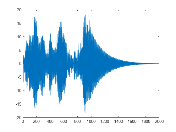
The mass is driven by random input for half of the measurement interval. Use the state-space model to compute the time evolution of the system starting from an all-zero initial state. Plot the acceleration of the mass as a function of time.

rng default

u = zeros(1,N);
u(1:N/2) = randn(1,N/2);

y = 0;
x = [0;0];
for k = 1:N
    y(k) = C*x + D*u(k);
    x = A*x + B*u(k);
end

plot(t,y)

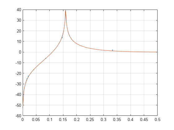
Estimate the transfer function of the system as a function of frequency. Use 2048 DFT points and specify a Kaiser window with a shape factor of 15. Use the default value of overlap between adjoining segments.

nfs = 2048;
wind = kaiser(N,15);

[txy,ft] = tfestimate(u,y,wind,[],nfs,Fs);

The frequency-response function of a discrete-time system can be expressed as the Z-transform of the time-domain transfer function of the system, evaluated at the unit circle. Verify that the estimate computed by tfestimate coincides with this definition.

[b,a] = ss2tf(A,B,C,D);

fz = 0:1/nfs:1/2-1/nfs;
z = exp(2j*pi*fz);
frf = polyval(b,z)./polyval(a,z);

plot(ft,20*log10(abs(txy)))
hold on
plot(fz,20*log10(abs(frf)))
hold off
grid
ylim([-60 40])

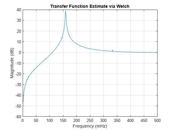
Plot the estimate using the built-in functionality of tfestimate.

tfestimate(u,y,wind,[],nfs,Fs)

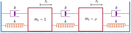
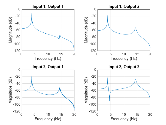
Estimate the transfer function for a multi-input/multi-output (MIMO) system.

Two masses connected to a spring and a damper on each side form an ideal one-dimensional discrete-time oscillating system. The system input array u consists of random driving forces applied to the masses. The system output array y contains the observed displacements of the masses from their initial reference positions. The system is sampled at a rate Fs of 40 Hz.

Load the data file containing the MIMO system inputs, the system outputs, and the sample rate. The example Frequency-Response Analysis of MIMO System analyzes the system that generated the data used in this example.

load MIMOdata

Estimate and plot the frequency-domain transfer functions of the system using the system data and the function tfestimate. Select the 'mimo' option to produce all four transfer functions. Use 214 sampling points to calculate the discrete Fourier transform, divide the signal into 5000-sample segments, and window each segment with a Hann window. Specify 2500 samples of overlap between adjoining segments.

wind = hann(5000);
nfs = 2^14;
nov = 2500;

[tXY,ft] = tfestimate(u,y,wind,nov,nfs,Fs,"mimo");

tiledlayout flow
for jk = 1:2
    for kj = 1:2
        nexttile
        plot(ft,mag2db(abs(tXY(:,jk,kj))))
        grid on
        ylim([-120 0])
        title("Input "+jk+", Output "+kj)
        xlabel("Frequency (Hz)")
        ylabel("Magnitude (dB)")
    end
end
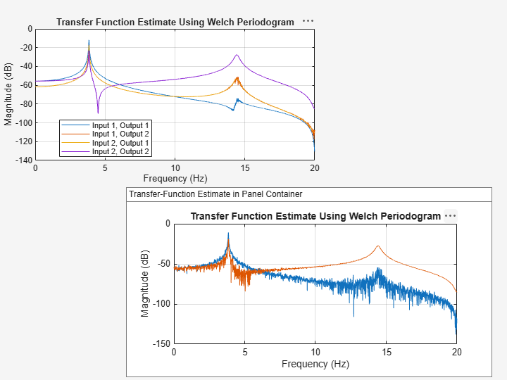
Input Arguments

collapse all

Input signal, specified as a vector or matrix.

Example: cos(pi/4*(0:159))+randn(1,160) specifies a sinusoid embedded in white Gaussian noise.

Data Types: single | double
Complex Number Support: Yes

Output signal, specified as a vector or matrix.

Data Types: single | double
Complex Number Support: Yes

Window, specified as an integer or as a row or column vector. Use window to divide the signal into segments.

  • If window is an integer, then tfestimate divides x and y into segments of length window and windows each segment with a Hamming window of that length.

  • If window is a vector, then tfestimate divides x and y into segments of the same length as the vector and windows each segment using window.

If the length of x and y cannot be divided exactly into an integer number of segments with noverlap overlapping samples, then the signals are truncated accordingly.

If you specify window as empty, then tfestimate uses a Hamming window such that x and y are divided into eight segments with noverlap overlapping samples.

For a list of available windows, see Windows.

Example: hann(N+1) and (1-cos(2*pi*(0:N)'/N))/2 both specify a Hann window of length N + 1.

Data Types: single | double

Number of overlapped samples, specified as a positive integer.

  • If window is scalar, then noverlap must be smaller than window.

  • If window is a vector, then noverlap must be smaller than the length of window.

If you specify noverlap as empty, then tfestimate uses a number that produces 50% overlap between segments.

Data Types: double | single

Number of DFT points, specified as a positive integer. If you specify nfft as empty, then tfestimate sets this argument to max(256,2p), where p = ⌈log2 N for input signals of length N and the ⌈ ⌉ symbols denote the ceiling function.

Data Types: single | double

Sample rate, specified as a positive scalar. The sample rate is the number of samples per unit time. If the unit of time is seconds, then the sample rate has units of Hz.

Normalized frequencies, specified as a row or column vector with at least two elements. Normalized frequencies are in rad/sample.

Example: w = [pi/4 pi/2]

Data Types: double | single

Frequencies, specified as a row or column vector with at least two elements. The frequencies are in cycles per unit time. The unit time is specified by the sample rate, fs. If fs has units of samples/second, then f has units of Hz.

Example: fs = 1000; f = [100 200]

Data Types: double | single

Frequency range for the transfer function estimate, specified as a one of 'onesided', 'twosided', or 'centered'. The default is 'onesided' for real-valued signals and 'twosided' for complex-valued signals.

  • 'onesided' — Returns the one-sided estimate of the transfer function between two real-valued input signals, x and y. If nfft is even, txy has nfft/2 + 1 rows and is computed over the interval [0,π] rad/sample. If nfft is odd, txy has (nfft + 1)/2 rows and the interval is [0,π) rad/sample. If you specify fs, the corresponding intervals are [0,fs/2] cycles/unit time for even nfft and [0,fs/2) cycles/unit time for odd nfft.

  • 'twosided' — Returns the two-sided estimate of the transfer function between two real-valued or complex-valued input signals, x and y. In this case, txy has nfft rows and is computed over the interval [0,2π) rad/sample. If you specify fs, the interval is [0,fs) cycles/unit time.

  • 'centered' — Returns the centered two-sided estimate of the transfer function between two real-valued or complex-valued input signals, x and y. In this case, txy has nfft rows and is computed over the interval (–π,π] rad/sample for even nfft and (–π,π) rad/sample for odd nfft. If you specify fs, the corresponding intervals are (–fs/2, fs/2] cycles/unit time for even nfft and (–fs/2, fs/2) cycles/unit time for odd nfft.

Transfer function estimator, specified as 'H1' or 'H2'.

  • Use 'H1' when the noise is uncorrelated with the input signals.

  • Use 'H2' when the noise is uncorrelated with the output signals. In this case, the number of input signals must equal the number of output signals.

See Transfer Function for more information.

Output Arguments

collapse all

Transfer function estimate, returned as a vector, matrix, or three-dimensional array.

Normalized frequencies, returned as a real-valued column vector.

Cyclical frequencies, returned as a real-valued column vector.

More About

collapse all

Transfer Function

The relationship between the input x and output y is modeled by the linear, time-invariant transfer function txy. In the frequency domain, Y(f) = H(f)X(f).

  • For a single-input/single-output system, the H1 estimate of the transfer function is given by

    H1(f)=Pyx(f)Pxx(f),

    where Pyx is the cross power spectral density of x and y, and Pxx is the power spectral density of x. This estimate assumes that the noise is not correlated with the system input.

    For multi-input/multi-output (MIMO) systems, the H1 estimator becomes

    H1(f)=PYX(f)PXX1(f)=[Py1x1(f)Py1x2(f)Py1xm(f)Py2x1(f)Py2x2(f)Py2xm(f)Pynx1(f)Pynx2(f)Pynxm(f)][Px1x1(f)Px1x2(f)Px1xm(f)Px2x1(f)Px2x2(f)Px2xm(f)Pxmx1(f)Pxmx2(f)Pxmxm(f)]1

    for m inputs and n outputs, where:

    • Pyixk is the cross power spectral density of the kth input and the ith output.

    • Pxixk is the cross power spectral density of the kth and ith inputs.

    For two inputs and two outputs, the estimator is the matrix

    H1(f)=[Py1x1(f)Px2x2(f)Py1x2(f)Px2x1(f)Py1x2(f)Px1x1(f)Py1x1(f)Px1x2(f)Py2x1(f)Px2x2(f)Py2x2(f)Px2x1(f)Py2x2(f)Px1x1(f)Py2x1(f)Px1x2(f)]Px1x1(f)Px2x2(f)Px1x2(f)Px2x1(f).

  • For a single-input/single-output system, the H2 estimate of the transfer function is given by

    H2(f)=Pyy(f)Pxy(f),

    where Pyy is the power spectral density of y and Pxy = P*yx is the complex conjugate of the cross power spectral density of x and y. This estimate assumes that the noise is not correlated with the system output.

    For MIMO systems, the H2 estimator is well-defined only for equal numbers of inputs and outputs: n = m. The estimator becomes

    H2(f)=PYY(f)PXY1(f)=[Py1y1(f)Py1y2(f)Py1yn(f)Py2y1(f)Py2y2(f)Py2yn(f)Pyny1(f)Pyny2(f)Pynyn(f)][Px1y1(f)Px1y2(f)Px1yn(f)Px2y1(f)Px2y2(f)Px2yn(f)Pxny1(f)Pxny2(f)Pxnyn(f)]1,

    where:

    • Pyiyk is the cross power spectral density of the kth and ith outputs.

    • Pxiyk is the complex conjugate of the cross power spectral density of the ith input and the kth output.

Algorithms

tfestimate uses Welch's averaged periodogram method. See pwelch for details.

References

[1] Vold, Håvard, John Crowley, and G. Thomas Rocklin. “New Ways of Estimating Frequency Response Functions.” Sound and Vibration. Vol. 18, November 1984, pp. 34–38.

Extended Capabilities

Version History

Introduced before R2006a

expand all