mscohere

Magnitude-squared coherence

Syntax

cxy = mscohere(x,y)

cxy = mscohere(x,y,window)

cxy = mscohere(x,y,window,noverlap)

cxy = mscohere(x,y,window,noverlap,nfft)

cxy = mscohere(___,"mimo")

[cxy,w] = mscohere(___)

[cxy,f] = mscohere(___,Fs)

[cxy,w] = mscohere(x,y,window,noverlap,w)

[cxy,f] = mscohere(x,y,window,noverlap,f,Fs)

[___] = mscohere(x,y,___,freqRange)

[___] = mscohere(___,Parent=h)

mscohere(___)

Description

cxy = mscohere(x,y) finds the magnitude-squared coherence estimate, cxy, of the input signals, x and y.

• If x and y are both vectors, they must have the same length.

• If one of the signals is a matrix and the other is a vector, then the length of the vector must equal the number of rows in the matrix. The function expands the vector and returns a matrix of column-by-column magnitude-squared coherence estimates.

• If x and y are matrices with the same number of rows but different numbers of columns, then mscohere returns a multiple coherence matrix. The mth column of cxy contains an estimate of the degree of correlation between all the input signals and the mth output signal. See Magnitude-Squared Coherence for more information.

• If x and y are matrices of equal size, then mscohere operates column-wise: cxy(:,n) = mscohere(x(:,n),y(:,n)). To obtain a multiple coherence matrix, append "mimo" to the argument list.

cxy = mscohere(x,y,window) uses window to divide x and y into segments and perform windowing. You must use at least two segments. Otherwise, the magnitude-squared coherence is 1 for all frequencies. In the MIMO case, the number of segments must be greater than the number of input channels.

cxy = mscohere(x,y,window,noverlap) uses noverlap samples of overlap between adjoining segments.

cxy = mscohere(x,y,window,noverlap,nfft) uses nfft sampling points to calculate the discrete Fourier transform.

cxy = mscohere(___,"mimo") computes a multiple coherence matrix for matrix inputs. This syntax can include any combination of input arguments from previous syntaxes.

[cxy,w] = mscohere(___) returns a vector of normalized frequencies, w, at which the magnitude-squared coherence is estimated.

[cxy,f] = mscohere(___,Fs) returns a vector of frequencies, f, expressed in terms of the sample rate, Fs, at which the magnitude-squared coherence is estimated. Fs must be the sixth numeric input to mscohere. To input a sample rate and still use the default values of the preceding optional arguments, specify these arguments as empty, [].

[cxy,w] = mscohere(x,y,window,noverlap,w) returns the magnitude-squared coherence estimate at the normalized frequencies specified in w.

[cxy,f] = mscohere(x,y,window,noverlap,f,Fs) returns the magnitude-squared coherence estimate at the frequencies specified in f.

[___] = mscohere(x,y,___,freqRange) returns the magnitude-squared coherence estimate over the frequency range specified by freqRange. Valid options for freqRange are "onesided", "twosided", and "centered".

[___] = mscohere(___,Parent=h) plots the magnitude-squared coherence estimate in the target parent container h. (since R2026a)

mscohere(___) with no output arguments plots the magnitude-squared coherence estimate in the current figure window.

Examples

Coherence Estimate of Two Sequences

Compute and plot the coherence estimate between two colored noise sequences.

Generate a signal consisting of white Gaussian noise. Reset the random number generator for reproducible results.

rng("default")
r = randn(16384,1);

To create the first sequence, bandpass filter the signal. Design a 16th-order filter that passes normalized frequencies between 0.2π and 0.4π rad/sample. Specify a stopband attenuation of 60 dB. Filter the original signal.

dx = designfilt("bandpassiir",FilterOrder=16, ...
    StopbandFrequency1=0.2,StopbandFrequency2=0.4, ...
    StopbandAttenuation=60);
x = filter(dx,r);

To create the second sequence, design a 16th-order filter that stops normalized frequencies between 0.6π and 0.8π rad/sample. Specify a passband ripple of 0.1 dB. Filter the original signal.

dy = designfilt("bandstopiir",FilterOrder=16, ...
    PassbandFrequency1=0.6,PassbandFrequency2=0.8, ...
    PassbandRipple=0.1);
y = filter(dy,r);

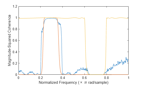
Estimate the magnitude-squared coherence of x and y. Use a 512-sample Hamming window. Specify 500 samples of overlap between adjoining segments and 2048 DFT points.

[cxy,fc] = mscohere(x,y,hamming(512),500,2048);

Plot the coherence function and overlay the frequency responses of the filters.

[qx,f] = freqz(dx);
qy = freqz(dy);

plot(fc/pi,cxy)
hold on
plot(f/pi,abs(qx),f/pi,abs(qy))
hold off
xlabel("Normalized Frequency (\times \pi rad/sample)")
ylabel("Magnitude-Squared Coherence")

Multiple Coherence and Ordinary Coherence

Specify a 30th-order FIR filter with a cutoff frequency of 0.3π and designed using a rectangular window. Generate a random two-channel signal, x. Generate another signal, y, by lowpass filtering the two channels and adding them together. Reset the random number generator for reproducible results.

h = fir1(30,0.3,rectwin(31));

rng("default")
x = randn(16384,2);
y = sum(filter(h,1,x),2);

Compute the multiple-coherence estimate of x and y. Window the signals with a 1024-sample Hann window. Specify 512 samples of overlap between adjoining segments and 1024 DFT points. Plot the estimate.

noverlap = 512;
nfft = 1024;

mscohere(x,y,hann(nfft),noverlap,nfft,"mimo")

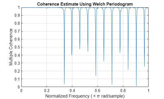
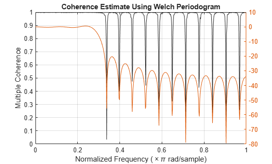
Compare the coherence estimate to the frequency response of the filter. The drops in coherence correspond to the zeros of the frequency response.

[H,f] = freqz(h);

hold on
yyaxis right
plot(f/pi,mag2db(abs(H)))
hold off

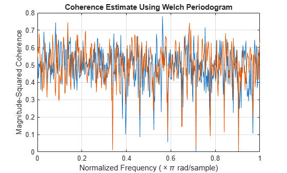
Compute and plot the ordinary magnitude-squared coherence estimate of x and y. The estimate does not reach 1 for any of the channels.

figure
mscohere(x,y,hann(nfft),noverlap,nfft)

Coherence of MIMO System

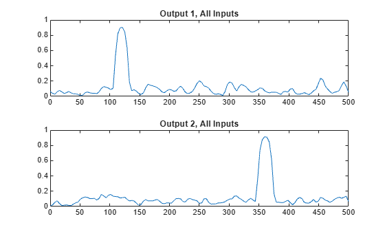
Generate two multichannel signals, each sampled at 1 kHz for 2 seconds. The first signal, the input, consists of three sinusoids with frequencies of 120 Hz, 360 Hz, and 480 Hz. The second signal, the output, is composed of two sinusoids with frequencies of 120 Hz and 360 Hz. One of the sinusoids lags the first signal by π/2. The other sinusoid has a lag of π/4. Both signals are embedded in white Gaussian noise. Reset the random number generator for reproducible results.

rng("default")

Fs = 1000;
f = 120;
t = (0:1/Fs:2-1/Fs)';

inpt = sin(2*pi*f*[1 3 4].*t);
inpt = inpt + randn(size(inpt));
oupt = sin(2*pi*f*[1 3].*t-[pi/2 pi/4]);
oupt = oupt + randn(size(oupt));

Estimate the degree of correlation between all the input signals and each of the output channels. Use a Hamming window of length 100 to window the data. mscohere returns one coherence function for each output channel. The coherence functions reach maxima at the frequencies shared by the input and the output.

[Cxy,f] = mscohere(inpt,oupt,hamming(100),[],[],Fs,"mimo");

for k = 1:size(oupt,2)
    subplot(size(oupt,2),1,k)
    plot(f,Cxy(:,k))
    title("Output " + k + ", All Inputs")
end

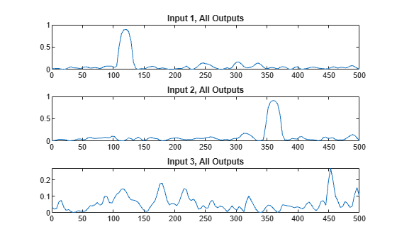
Switch the input and output signals and compute the multiple coherence function. Use the same Hamming window. There is no correlation between input and output at 480 Hz. Thus there are no peaks in the third correlation function.

[Cxy,f] = mscohere(oupt,inpt,hamming(100),[],[],Fs,"mimo");

for k = 1:size(inpt,2)
    subplot(size(inpt,2),1,k)
    plot(f,Cxy(:,k))
    title("Input " + k + ", All Outputs")
end

Repeat the computation, using the plotting functionality of mscohere.

clf
mscohere(oupt,inpt,hamming(100),[],[],Fs,"mimo")

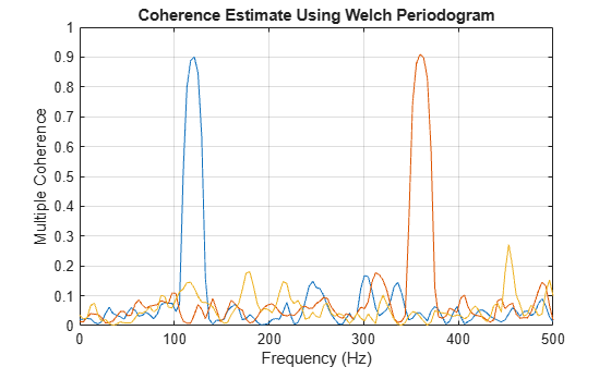
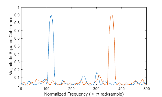
Compute the ordinary coherence function of the second signal and the first two channels of the first signal. The off-peak values differ from the multiple coherence function.

[Cxy,f] = mscohere(oupt,inpt(:,[1 2]),hamming(100),[],[],Fs);
plot(f,Cxy)
xlabel("Normalized Frequency (\times \pi rad/sample)")
ylabel("Magnitude-Squared Coherence")

Find the phase differences by computing the angle of the cross-spectrum at the points of maximum coherence.

Pxy = cpsd(oupt,inpt(:,[1 2]),hamming(100),[],[],Fs);
[~,mxx] = max(Cxy);
for k = 1:2
    fprintf("Phase lag %d = %5.2f*pi\n",k,angle(Pxy(mxx(k),k))/pi)
end

Phase lag 1 = -0.51*pi
Phase lag 2 = -0.22*pi

Modify Magnitude-Squared Coherence Plot

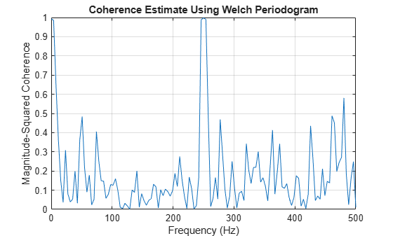
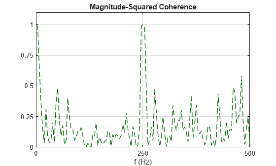
Generate two sinusoidal signals sampled for 1 second each at 1 kHz. Each sinusoid has a frequency of 250 Hz. One of the signals lags the other in phase by π/3 radians. Embed both signals in white Gaussian noise of unit variance.

rng("default")

Fs = 1000;
f = 250;
t = 0:1/Fs:1-1/Fs;
um = sin(2*pi*f*t) + rand(size(t));
un = sin(2*pi*f*t-pi/3) + rand(size(t));

Use mscohere to compute and plot the magnitude-squared coherence of the signals.

mscohere(um,un,[],[],[],Fs)

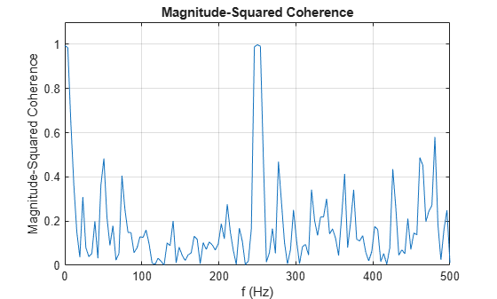
Modify the title of the plot, the label of the x-axis, and the limits of the y-axis.

title("Magnitude-Squared Coherence")
xlabel("f (Hz)")
ylim([0 1.1])

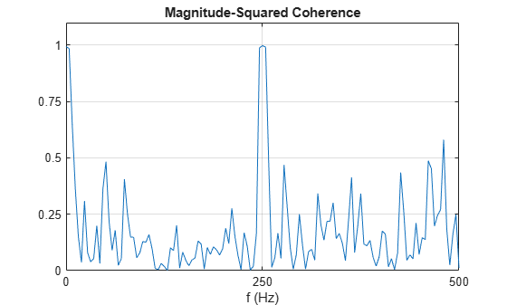
Use gca to obtain a handle to the current axes. Change the locations of the tick marks. Remove the label of the y-axis.

ax = gca;
ax.XTick = 0:250:500;
ax.YTick = 0:0.25:1;
ax.YLabel.String = [];

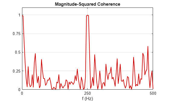
Call the Children property of the handle to change the color and width of the plotted line.

ln = ax.Children;
ln.Color = [0.8 0 0];
ln.LineWidth = 1.5;

Alternatively, use set and get to modify the line properties.

set(get(gca,"Children"),Color=[0 0.4 0],LineStyle="--",LineWidth=1)

Plot Magnitude-Squared Coherence Estimate of MIMO System in Target Parent Container

Since R2026a

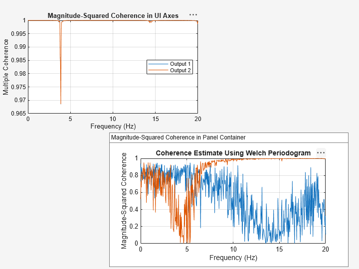
Plot the magnitude-squared coherence estimate for a MIMO system in the specified target axes and panel containers.

Two masses connected to a spring and a damper on each side form an ideal one-dimensional discrete-time oscillating system. The system input array u consists of random driving forces applied to the masses. The system output array y contains the observed displacements of the masses from their initial reference positions. The system is sampled at a rate Fs of 40 Hz.

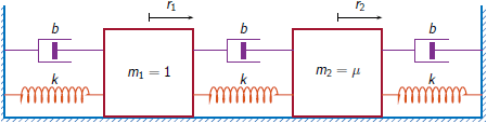
Load the data file containing the MIMO system inputs, the system outputs, and the sample rate. The example Frequency-Response Analysis of MIMO System analyzes the system that generated the data used in this example.

load MIMOdata Fs u y

Estimate the magnitude-squared coherence of the system and plot the estimate on a UI axes. Divide the signal into 5000-sample segments with 50% overlap between adjoining segments. Apply a Hanning window to each segment and calculate the discrete Fourier transform of the signal segment using 1024 frequency points. Select the "mimo" option to produce the multiple-coherence estimates.

uif = uifigure(Position=[100 100 720 540]);
ax = uiaxes(uif,Position=[5 280 400 240]);

g = hann(5000);
ol = 2500;
nfft = 1024;

mscohere(u,y,g,ol,nfft,Fs,"mimo",Parent=ax)
legend(ax,"Output "+[1 2]',Location="best")
title(ax,"Magnitude-Squared Coherence in UI Axes")

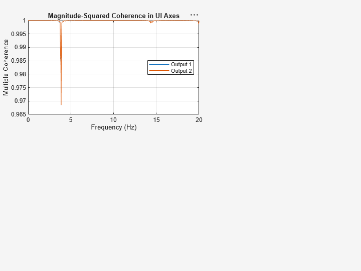
Add a panel container in the southeastern corner of the UI figure window.

p = uipanel(uif,Position=[220 5 480 270], ...
    Title="Magnitude-Squared Coherence in Panel Container", ...
    BackgroundColor="white");

Plot the magnitude-squared coherence estimate of each input-output pair of the system.

mscohere(u,y,g,ol,nfft,Fs,Parent=p)

Input Arguments

x, y — Input signals

vectors | matrices

Input signals, specified as vectors or matrices.

Example: cos(pi/4*(0:159))+randn(1,160) specifies a sinusoid embedded in white Gaussian noise.

Data Types: single | double
Complex Number Support: Yes

window — Window

integer | vector | []

Window, specified as an integer or as a row or column vector. Use window to divide the signal into segments:

• If window is an integer, then mscohere divides x and y into segments of length window and windows each segment with a Hamming window of that length.

• If window is a vector, then mscohere divides x and y into segments of the same length as the vector and windows each segment using window.

If the length of x and y cannot be divided exactly into an integer number of segments with noverlap overlapping samples, then the signals are truncated accordingly.

If you specify window as empty, then mscohere uses a Hamming window such that x and y are divided into eight segments with noverlap overlapping samples.

For a list of available windows, see Windows.

Example: hann(N+1) and (1-cos(2*pi*(0:N)'/N))/2 both specify a Hann window of length N + 1.

Data Types: single | double

noverlap — Number of overlapped samples

positive integer | []

Number of overlapped samples, specified as a positive integer.

• If window is scalar, then noverlap must be smaller than window.

• If window is a vector, then noverlap must be smaller than the length of window.

If you specify noverlap as empty, then mscohere uses a number that produces 50% overlap between segments. If the segment length is unspecified, the function sets noverlap to ⌊N/4.5⌋, where N is the length of the input and output signals.

Data Types: double | single

nfft — Number of DFT points

positive integer | []

Number of DFT points, specified as a positive integer. If you specify nfft as empty, then mscohere sets this argument to max(256,2^p), where p = ⌈log₂ N⌉ for input signals of length N.

Data Types: single | double

Fs — Sample rate

positive scalar

Sample rate, specified as a positive scalar. The sample rate is the number of samples per unit time. If the unit of time is seconds, then the sample rate is in Hz.

• If you specify Fs as empty [], then mscohere assumes that the input signal x has a sample rate of 1 Hz.

• If you do not specify Fs, then mscohere assumes that the input signal x has a sample rate of 2π rad/sample.

w — Normalized frequencies

vector

Normalized frequencies, specified as a row or column vector with at least two elements. Normalized frequencies are in rad/sample.

Example: w = [pi/4 pi/2]

Data Types: double | single

f — Frequencies

vector

Frequencies, specified as a row or column vector with at least two elements. The frequencies are in cycles per unit time. The unit time is specified by the sample rate, fs. If fs has units of samples/second, then f has units of Hz.

Example: fs = 1000; f = [100 200]

Data Types: double | single

freqRange — Frequency range for magnitude-squared coherence estimate

"onesided" | "twosided" | "centered"

Frequency range for the magnitude-squared coherence estimate, specified as "onesided", "twosided", or "centered". The default is "onesided" for real-valued signals and "twosided" for complex-valued signals.

• "onesided" — Returns the one-sided estimate of the magnitude-squared coherence estimate between two real-valued input signals, x and y. If nfft is even, cxy has nfft/2 + 1 rows and is computed over the interval [0,π] rad/sample. If nfft is odd, cxy has (nfft + 1)/2 rows and the interval is [0,π) rad/sample. If you specify Fs, the corresponding intervals are [0,Fs/2] cycles/unit time for even nfft and [0,Fs/2) cycles/unit time for odd nfft.

• "twosided" — Returns the two-sided estimate of the magnitude-squared coherence estimate between two real-valued or complex-valued input signals, x and y. In this case, cxy has nfft rows and is computed over the interval [0,2π) rad/sample. If you specify Fs, the interval is [0,Fs) cycles/unit time.

• "centered" — Returns the centered two-sided estimate of the magnitude-squared coherence estimate between two real-valued or complex-valued input signals, x and y. In this case, cxy has nfft rows and is computed over the interval (–π,π] rad/sample for even nfft and (–π,π) rad/sample for odd nfft. If you specify Fs, the corresponding intervals are (–Fs/2, Fs/2] cycles/unit time for even nfft and (–Fs/2, Fs/2) cycles/unit time for odd nfft.

If you specify a vector w or f of frequencies and freqRange as inputs, then mscohere ignores freqRange.

h — Target parent container

[] (default) | Axes object | UIAxes object | Panel object

Since R2026a

Target parent container, specified as an Axes object, a UIAxes object, or a Panel object.

If you specify Parent=h, the mscohere function plots the magnitude-squared coherence estimate on the specified target parent container, whether you call the function with or without output arguments.

For more information about target containers and the parent-child relationship in MATLAB^® graphics, see Graphics Object Hierarchy. For more information about using Parent in UIAxes and Panel objects to design apps, see Plot Spectral Representations of Signal in App Designer.

Example: h = axes(figure,Position=[0.1 0.1 0.6 0.5]) defines an axes parent container. When you specify mscohere(x,y,[],[],[],Parent=h), the function plots the magnitude-squared coherence estimate of the signals x and y in the parent container h.

Output Arguments

cxy — Magnitude-squared coherence estimate

vector | matrix | three-dimensional array

Magnitude-squared coherence estimate, returned as a vector, matrix, or three-dimensional array.

w — Normalized frequencies

vector

Normalized frequencies, returned as a real-valued column vector.

f — Frequencies

vector

Frequencies, returned as a real-valued column vector.

More About

Magnitude-Squared Coherence

The magnitude-squared coherence estimate is a function of frequency with values between 0 and 1. These values indicate how well x corresponds to y at each frequency. The magnitude-squared coherence is a function of the power spectral densities, P_xx(f) and P_yy(f), and the cross power spectral density, P_xy(f), of x and y:

$$C_{xy}(f)=\frac{{\left|P_{xy}(f)\right|}^2}{P_{xx}(f)P_{yy}(f)}.$$

For multi-input/multi-output systems, the multiple-coherence function becomes

$$\begin{array}{c}{C}_{X{y}_i}(f)=\frac{P_{X{y}_i}^{†}(f)P_{XX}^{-1}(f)P_{X{y}_i}(f)}{P_{y_i{y}_i}(f)}\\ =\left[\begin{array}{ccc}{P}_{x_1{y}_i}^{*}(f)& \cdots & P_{x_m{y}_i}^{*}(f)\end{array}\right]{\left[\begin{array}{cccc}{P}_{x_1{x}_1}(f)& P_{x_1{x}_2}(f)& \cdots & P_{x_1{x}_m}(f)\\ P_{x_2{x}_1}(f)& P_{x_2{x}_2}(f)& \cdots & P_{x_2{x}_m}(f)\\ ⋮& ⋮& \ddots & ⋮\\ P_{x_m{x}_1}(f)& P_{x_m{x}_2}(f)& \cdots & P_{x_m{x}_m}(f)\end{array}\right]}^{-1}\left[\begin{array}{c}{P}_{x_1{y}_i}(f)\\ ⋮\\ P_{x_m{y}_i}(f)\end{array}\right]\frac{1}{P_{y_i{y}_i}(f)}\end{array}$$

for the ith output signal, where:

• X corresponds to the array of m inputs.

• P_Xyi is the m-dimensional vector of cross power spectral densities between the inputs and y_i.

• P_XX is the m-by-m matrix of power spectral densities and cross power spectral densities of the inputs.

• P_yiyi is the power spectral density of the output.

• The dagger (†) stands for the complex conjugate transpose.

Algorithms

mscohere estimates the magnitude-squared coherence function [2] using Welch’s overlapped averaged periodogram method [3], [5].

References

[1] Gómez González, A., J. Rodríguez, X. Sagartzazu, A. Schumacher, and I. Isasa. “Multiple Coherence Method in Time Domain for the Analysis of the Transmission Paths of Noise and Vibrations with Non-Stationary Signals.” Proceedings of the 2010 International Conference of Noise and Vibration Engineering, ISMA2010-USD2010. pp. 3927–3941.

[2] Kay, Steven M. Modern Spectral Estimation. Englewood Cliffs, NJ: Prentice-Hall, 1988.

[3] Rabiner, Lawrence R., and Bernard Gold. Theory and Application of Digital Signal Processing. Englewood Cliffs, NJ: Prentice-Hall, 1975.

[4] Stoica, Petre, and Randolph Moses. Spectral Analysis of Signals. Upper Saddle River, NJ: Prentice Hall, 2005.

[5] Welch, Peter D. “The Use of Fast Fourier Transform for the Estimation of Power Spectra: A Method Based on Time Averaging Over Short, Modified Periodograms.” IEEE^® Transactions on Audio and Electroacoustics. Vol. AU-15, 1967, pp. 70–73.

Extended Capabilities

C/C++ Code Generation
Generate C and C++ code using MATLAB® Coder™.

GPU Code Generation
Generate CUDA® code for NVIDIA® GPUs using GPU Coder™.

GPU Arrays

Accelerate code by running on a graphics processing unit (GPU) using Parallel Computing Toolbox™.

This function fully supports GPU arrays. For more information, see Run MATLAB Functions on a GPU (Parallel Computing Toolbox).

Version History

Introduced before R2006a

R2026a: Visualize function outputs in specified parent targets

The mscohere function supports plotting output in a parent axes or panel container specified using the Parent input argument.

R2024a: Code generation support for single-precision variable-size window inputs

The mscohere function supports single-precision variable-size window inputs for code generation.

R2023b: Use single-precision data

The mscohere function supports single-precision inputs.