Helicopter Modeling and Simulation

Since R2024b

This example demonstrates how to model, simulate, control, and visualize a UH-1H helicopter system in Simulink® using the Rotor (Aerospace Blockset) and 6DOF (Euler Angles) (Aerospace Blockset) blocks from Aerospace Blockset™.

Model Overview

Open the Simulink® model.

mdl = "HelicopterModelingSimulation";
open_system(mdl);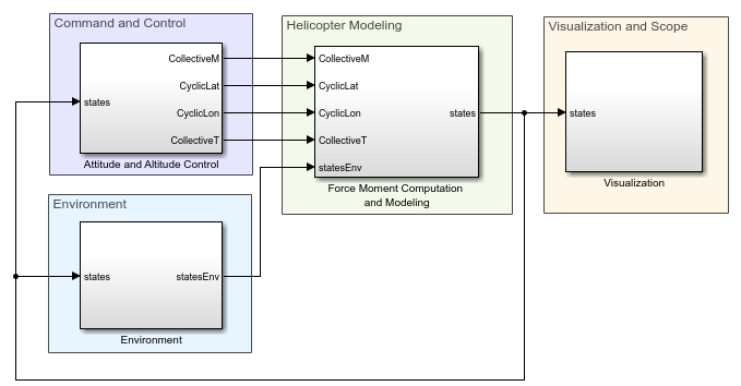

The top model consists of six subsystems:

1. Helicopter Model

2. Sensor

3. Input Panel

4. Environment

5. Command and Control

6. Visualization and Scope

Helicopter Model

This example models a helicopter by computing the forces and moments exerted by each part of helicopter and resolving them along the center of gravity of the helicopter. The resultant forces and moments are then fed to the 6DOF (Euler Angles) (Aerospace Blockset) block, which implements 6DOF equations of motion to simulate the helicopter model.

These components are included in the Force Moment Computation subsystem.

1. Main Rotor

2. Tail Rotor

3. Fuselage

4. Vertical Fin

5. Horizontal Stabilizer

6. Gravity

The UH-1H helicopter [1] parameters are used to compute forces and moments for the helicopter components. The helicopter weighs 2800 kg. For the purposes of this example, maintain constant speeds for the main rotor and tail rotor.

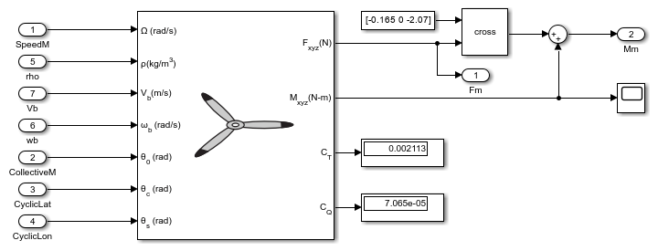
Main Rotor

A Rotor block models the main rotor of the helicopter by enabling the flap effects. The main rotor of the UH-1H helicopter is located at aft and above the CG position. Consequently, the moments from the Rotor block are resolved using the Cross Product block. The control input to the main rotor is the collective blade pitch angle, ${\theta }_0$, lateral cyclic pitch angle, ${\theta }_{\mathit{c}}$, and longitudinal cyclic pitch angle, ${\theta }_{\mathit{s}}$.

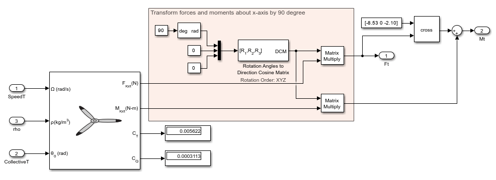
Tail Rotor

The tail rotor is modeled using the Rotor block without flap effects. Unlike the main rotor, the tail rotor is mounted vertically. Hence, the forces and moments from the Rotor block should be transformed about x-axis by 90 degrees, to properly represent its orientation. The Rotation Angles to Direction Cosine Matrix block carries out this transformation. As the tail rotor is located at aft and above the CG position of the helicopter system, the moments from the Rotor block are resolved using a Cross Product block. The control input to the tail rotor is the collective blade pitch angle, ${\theta }_0$, of the tail rotor.

Fuselage

This example uses simple fuselage aerodynamics of a UH-1H helicopter [1], implemented using a MATLAB Function block.

$${\mathit{X}}_{\mathit{F}}={\mathit{u}}_{\mathit{B}}\left(-{\mathit{D}}_1\left|{\mathit{u}}_{\mathit{B}}\right|+{\mathit{L}}_1\frac{{\mathit{w}}_{\mathit{B}}^2}{\left|{\mathit{u}}_{\mathit{B}}\right|}\right)=-{\mathit{D}}_1{\mathit{u}}_{\mathit{B}}\left|{\mathit{u}}_{\mathit{B}}\right|+{\mathit{L}}_1{\mathit{w}}_{\mathit{B}}^2\mathrm{sign}\left({\mathit{u}}_{\mathit{B}}\right)$$

${\mathit{Y}}_{\mathit{F}}={\mathit{v}}_{\mathit{B}}\left(-{\mathit{D}}_2\left|{\mathit{v}}_{\mathit{B}}\right|-{\mathit{Y}}_1\left|{\mathit{u}}_{\mathit{B}}\right|\right)$

${\mathit{Z}}_{\mathit{F}}={\mathit{w}}_{\mathit{B}}\left(-{\mathit{D}}_3\left|{\mathit{w}}_{\mathit{B}}\right|-{\mathit{L}}_1\left|{\mathit{u}}_{\mathit{B}}\right|\right)$

${\mathit{L}}_{\mathit{F}}=0$

${\mathit{M}}_{\mathit{F}}={\mathit{M}}_1{\mathit{w}}_{\mathit{B}}\left|{\mathit{u}}_{\mathit{B}}\right|$

$${\mathit{N}}_{\mathit{F}}={-\mathit{N}}_1{\mathit{v}}_{\mathit{B}}{\mathit{u}}_{\mathit{B}}$$

Vertical Fin

The vertical fin aerodynamics corresponding to the UH-1H helicopter [1] are implemented using a MATLAB Function block.

$${\mathit{u}}_{\mathit{v}}={\mathit{u}}_{\mathit{B}}$$

$${\mathit{v}}_{\mathit{v}}=-{\mathit{v}}_{\mathit{B}}+{\mathit{l}}_{\mathrm{VF}}{\mathit{r}}_{\mathit{B}}$$

$${\mathit{Y}}_{\mathit{v}}={\mathit{K}}_1{\mathit{v}}_{\mathit{v}}{\mathit{u}}_{\mathit{v}}+{\mathit{F}}_1{\mathit{v}}_{\mathit{v}}\left|{\mathit{v}}_{\mathit{v}}\right|$$

$${\mathit{N}}_{\mathit{v}}=-{\mathit{Y}}_{\mathit{v}}{\mathit{l}}_{\mathrm{VF}}$$

Horizontal Stabilizer

The aerodynamics corresponding to the horizontal stabilizer of the UH-1H helicopter [1] are implemented using a MATLAB Function block.

$${\mathit{u}}_{\mathit{H}}={\mathit{u}}_{\mathit{B}}$$

$${\mathit{w}}_{\mathit{H}}={\mathit{w}}_{\mathit{B}}+{\mathit{l}}_{\mathrm{HS}}{\mathit{q}}_{\mathit{B}}$$

$${\mathit{Z}}_{\mathit{H}}=-{\mathit{H}}_1{\mathit{w}}_{\mathit{H}}{\mathit{u}}_{\mathit{H}}-{\mathit{H}}_4{\mathit{w}}_{\mathit{H}}\left|{\mathit{w}}_{\mathit{H}}\right|$$

$${\mathit{M}}_{\mathit{H}}={\mathit{Z}}_{\mathit{H}}{\mathit{l}}_{\mathrm{HS}}$$

Gravity

The force due to gravity in the body axes frame is obtained by multiplying the Direction Cosine Matrix, DCM with the gravitational force vector defined in the North-East-Down (NED) frame.

Sensor

The Sensor subsystem simulates sensor outputs by perturbing the output of the 6DOF (Euler Angles) block with noise to represent measurement imperfections. This enables realistic testing of the control system’s robustness to noisy sensor data within the simulation environment.

Input Panel

The Input Panel subsystem acts as the user interface for setting reference commands to the helicopter system. It incorporates different variant subsystems to accommodate three maneuver modes. In the Path mode, users can specify the reference velocity, VRef, while the reference altitude is automatically determined based on user-defined waypoints. The Level mode enables users to manually set both the reference altitude, hRef and velocity, VRef. For the Hover mode, the reference altitude, hRef is set by the user.

Instrument Panel

The Instrument Panel subsystem visualizes key helicopter state variables using aircraft-specific gauges from the Aerospace Blockset™ Flight Instrumentation library. This subsystem provides a cockpit-like display, enabling users to monitor parameters such as altitude, velocity, and attitude in real time during simulation.

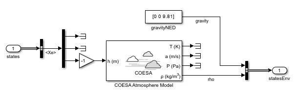
Environment

The Environment subsystem models the external conditions affecting helicopter flight. In this example, it assumes a constant gravitational acceleration of $9.81\mathit{m}/{\mathit{s}}^2$ and calculates air density as a function of altitude using the COESA Atmosphere Model (Aerospace Blockset) block.

Command and Control

The Command and Control subsystem manages and directs the behavior and responses of the helicopter. Since the helicopter is an underactuated system, where the number of control inputs is less than the number of states or modes to be controlled, this subsystem includes a cascaded proportional integral derivative (PID) control strategy.

This control mechanism is structured in a hierarchical manner, where multiple PID controllers are cascaded to refine the control action at each level. Each PID controller in the cascade is responsible for a specific aspect of the operation of the helicopter. For example, the inner loop controls the rate, and the outer loop controls the corresponding angle. This mechanism acts as an effective control strategy for an underactuated system.

Assuming constant rotor speeds, control inputs to the helicopter system include the collective blade pitch angle, and the lateral and longitudinal cyclic pitch angles. The collective blade pitch angle of the main rotor controls the altitude of the helicopter. The lateral cyclic pitch angle, the longitudinal cyclic pitch angle of the main rotor, and the collective blade pitch angle of the tail rotor control roll, pitch, and yaw motions, respectively.

The climb rate of the UH-1H helicopter is $488m/\min$, so the reference altitude increases at a rate of $8m/s$ until the helicopter reaches its desired altitude. The forward velocity is computed based on the specified velocity. You can assume that the lateral velocity is zero. The pitch and roll angle values are calculated by the PID controllers using the reference forward and lateral velocity values.

Visualization and Scope

The Visualization subsystem visualizes the helicopter in a simulation environment that uses the Unreal Engine® from Epic Games®. Visualization can be performed by co-simulation between Unreal Engine® and the Simulation 3D Scene Configuration (Aerospace Blockset), Helicopter (Aerospace Blockset), and Simulation 3D Rotorcraft (Aerospace Blockset) blocks. For more information on the Unreal Engine simulation environment, see How 3D Simulation for Aerospace Blockset Works (Aerospace Blockset).

To visualize the simulation results with Simulink 3D Animation, select the visual3D check box.

visual3D = false;

Run the live script to update the values, before executing the Simulink model.

Helicopter Simulation

Simulate the model to perform path-following, steady level-flight, or hover maneuvers. By default, the desired state is set to "path" to perform the path-following maneuver. To perform a level-flight or hover maneuver, choose the corresponding option from the dropdown.

state = "path";

Set the flying altitude of the helicopter. The maximum altitude of the UH-1H helicopter is $3500\mathit{m}$.

if state == "hover"||state == "level"
    hRef = 20;
end

For steady level-flight condition, set the desired velocity. The maximum velocity is $65m/s$ to represent the physical constraint of UH-1H helicopter.

if state == "level"
    VRef = 30;
end

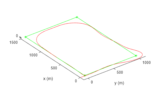
In this example, waypoints are used to guide the helicopter along a specific path. The choice of waypoints is used to define the trajectory and ensure that the helicopter follows the desired path during the simulation. Define the waypoints in the matrix WP, where each column represents a 3D coordinate in the format [x; y; z].

Ensure that each successive waypoint is defined at least 500 m apart, matching the 500 m lookahead distance. The guidance system calculates the yaw angle required to steer the aircraft on to the desired path. For information on guidance laws, see [2].

out = sim(mdl);

if state == "path"

    VRef = 30;
    WP(:,1) = [0; 0; -20];
    WP(:,2) = [1500; 0; -20];
    WP(:,3) = [1500; 1000; -20];
    WP(:,4) = [0; 1000; -20];
    WP(:,5) = [0; 0; -20];
    

Use the plot3 function to visualize the waypoints and the helicopter's path in a 3D space.

    plot3(WP(2,:),WP(1,:),WP(3,:),'g*')
    hold on
    plot3(WP(2,:),WP(1,:),WP(3,:),'g')
    axis equal
    plot3(out.posout.Data(:,2),out.posout.Data(:,1),out.posout.Data(:,3),'r')
    xlabel('y (m)');
    ylabel('x (m)');
else
    subplot(2,1,1)
    plot(out.posout.Time,-out.posout.Data(:,3))
    ylabel('Altitude (m)')
    subplot(2,1,2)
    plot(out.logsout{11}.Values.Time,out.logsout{11}.Values.Data)
    xlabel('Time (s)');
    ylabel('Airspeed (m/s)');
end

The desired altitude of the helicopter is controlled with a PID controller, by using the collective pitch angle of the main rotor as input. Calculate the desired roll angle and pitch angle using the PID controller, based on the desired ${\mathit{v}}_{\mathit{B}}$ and ${\mathit{u}}_{\mathit{B}}$, respectively. You can calculate the desired yaw angle by applying the guidance laws in [2]. Control the roll, pitch, and yaw angles with cascaded PID controllers, utilizing corresponding rate controls p, q, and r in the inner loop. Use the lateral cyclic and longitudinal cyclic pitch angles of the main rotor for roll and pitch control and the collective pitch angle of the tail rotor for yaw control.

Reference

[1] Talbot, Peter D. and Lloyd D. Corliss. "A Mathematical Force and Moment Model of a UH-1H Helicopter for Flight Dynamics Simulations." NASA Ames Research Center, 1977. https://ntrs.nasa.gov/archive/nasa/casi.ntrs.nasa.gov/19770024231.pdf

[2] Fossen, T. I. "An Adaptive Line-of-Sight (ALOS) Guidance Law for Path Following of Aircraft and Marine Craft." IEEE Transactions on Control Systems Technology 31, no. 6 (November 2023): 2887–2894. https://doi.org/10.1109/TCST.2023.3259819.