Intelligent PID using Ultra Local Model for Ball on Beam Balance

This example shows how to implement a model-free control technique called intelligent PID (iPID) using the Ultra-Local Model (ULM) block in Simulink®. The Ultra-Local Model block is used to estimates a local linear and control affine model of the plant. The iPID controller use a baseline PID controller plus and synthesizes ULM estimate to enable reference tracking for the system with model uncertainties and/or external disturbances.

Ball and Beam Balance Model

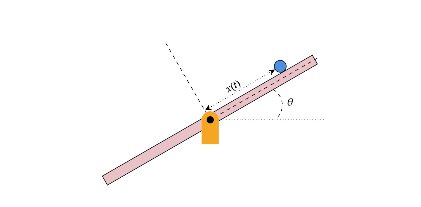
This example shows how to implement an iPID controller for a challenging task of balancing a ball on a beam. The ball and beam system involves a ball placed on beam free to move along the length of beam with 1-degree of freedom. The beam itself can rotate as shown in the figure. When the beam rotates from its horizontal position, the gravity causes the ball to roll along the beam. This example aims to design a controller to control the position of the ball on the beam.

The equation of motion of the ball on the beam is as follows:

$$\left(\frac{\mathit{J}}{{\mathit{R}}^2}+\mathit{m}\right)\ddot{\mathit{x}}=\mathit{mx}{\dot{\theta }}^2-\mathit{mgsin}\left(\theta \right)$$

where

• $\mathit{m}:$ Mass of the ball

• $\mathit{R}:$ Radius of the ball

• $\mathit{J}:$ Moment if inertia of the ball

• $\mathit{x}:$ Coordinate of the ball along the beam

• $\theta :$ Beam angle of rotation

The ball position $\mathit{y}=\mathit{x}\left(\mathit{t}\right)$ is the plant output and beam angle $\mathit{u}=\theta \left(\mathit{t}\right)$ is the control input to the plant.

Define the physical properties of ball and beam.

m = 0.11;    % Mass of the ball (kg)
R = 0.015;   %Radius of the ball (m)
J = 9.99e-6; % Ball moment of Inertia(kgm^2)

g = 9.8;     %Gravitational constant (m/s^2)

% Define variable 'B' 

B = m/(J/R^2+m);

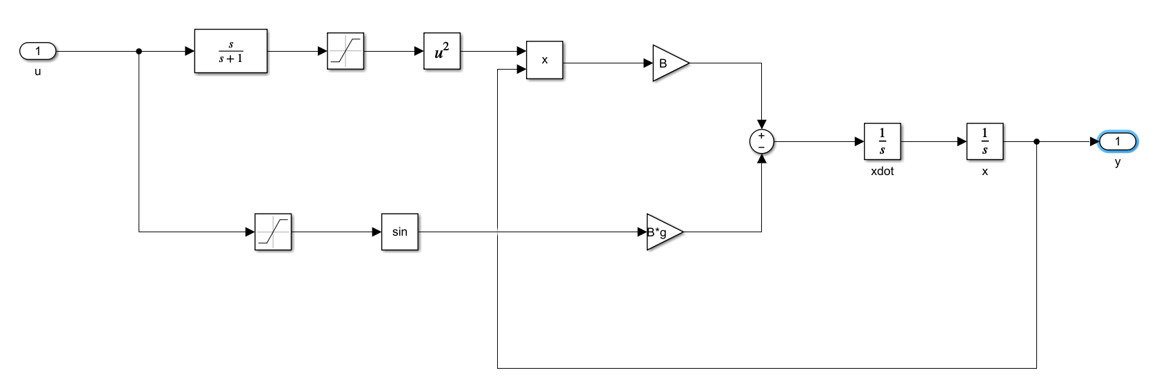
The ball and beam model is implemented in Simulink® as shown in this figure.

Controller Objective

The objective of controller is to make the ball track a given reference trajectory. The ball starts at rest from position at $\mathit{x}=0$. The control input to the system is tilt angle of the beam. The aim is to track a sinusoidal reference. The system is open-loop unstable, without any active control the ball rolls off the beam, hence an active controller is necessary to control the ball's position on the beam.

To begin with, this example implements the most popular fixed gain Proportional-Integral-Derivative (PID) controller for this task.

To simulate the ball balance on beam example, open the Simulink model,

mdl = 'iPIDBallandBeamUsingULM';
open_system(mdl)

Select the PID as controller of choice

% Set '0' for PID and '1' for iPID
usePID = '0';
useIntelligentPID = '1';

% Select the baseline PID controller
set_param([mdl,'/pid on-off'],'sw',usePID)

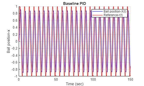
The baseline controller is tuned using the PID Tuner app. Run the model to simulate the ball and beam example with baseline controller.

out = sim(mdl);

Plot the simulation results

fig1 = figure();
hold on
grid on
plot(out.tout,out.y.Data,'b')
plot(out.tout,out.r.Data,'r')
xlabel('Time (sec)')
ylabel('Ball position-x')
legend('Ball position-X(t)','Reference-r(t)')
title('Baseline PID')

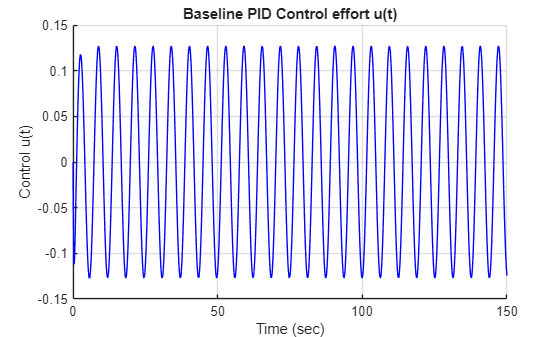
Plot the PID control effort

% Plot the control effort
fig2 = figure();
hold on
grid on
plot(out.tout,out.u.Data,'b')
xlabel('Time (sec)')
ylabel('Control u(t)')
title('Baseline PID Control effort u(t)')

The tuned PID controller has large tracking error and does not meet the tracking requirement satisfactorily. This is mainly due to nonlinear nature of the system which is not captured well with linear approximation of the plant. Hence, the system requires a controller technique which can account for the disturbance caused by unmodeled dynamics. The next section discusses such a technique that implement model-free control using ultra-local model augmented PID.

Model-Free Control

This section briefly introduces the topic of model-free control using Ultra-Local Model, and further discuss how you can augment a baseline controller like PID with ULM estimates to build a data driven intelligent PID [1].

Ultra-Local Model Overview

Ultra-Local Model is a simplified local linear model updated via the unique knowledge of the input-output behavior. The control affine linear ULM is defined as follows

$${\mathit{y}}^{\left(\mathit{n}\right)}=\mathit{F}+\alpha \mathit{u}$$

where $\mathit{n},\alpha$ are tunable parameters

1. $\mathit{n}\in \left[1,2\right]$ is the derivation order of ULM model

2. The time-varying quantity $\mathit{F}$ subsumes not only the un-modeled dynamics, but also the external disturbances.

3. the constant $\alpha \in \mathit{R}$ is input gain and is chosen such that the three quantities ${\mathit{y}}^{\left(\mathit{n}\right)},\mathit{F}\mathrm{and}\alpha \mathit{u}$ are of the same order of magnitude.

The ULM model is identified online using first-order or second order Algebraic methods, see Ultra-Local Model for Disturbance Estimation and Compensation.

Model-Free Control Law Using ULM

Ultra-Local Model technique have been applied to perform Model-Free Control (MFC) of nonlinear systems with unknown or partially known dynamics. MFC synthesize local estimates of lumped unknown provided by the ULM model with a baseline control and feedforward control to come-up with a total controller.

The model free controller is of the form

$$\mathit{u}\left(\mathit{t}\right)=-\frac{\mathit{F}\left(\mathit{t}\right)}{\alpha }+\frac{{\mathit{y}}_{\mathit{d}}^{\left(\mathit{n}\right)}-{\mathit{u}}_{\mathit{c}}\left(\mathit{e}\left(\mathit{t}\right)\right)}{\alpha }$$

where

• $\mathit{u}\left(\mathit{t}\right):$ Total control

• $\mathit{F}\left(\mathit{t}\right):$ Estimate of the lumped plant uncertainties/disturbances.

• ${\mathit{y}}_{\mathit{d}}^{\left(\mathit{n}\right)}:$ nth order derivative of reference

• ${\mathit{u}}_{\mathit{c}}\left(\mathit{e}\left(\mathit{t}\right)\right):$ Stabilizing feedback control that should be selected in a way to guarantee asymptotic convergence of the output signal to the desired trajectory.

• $\mathit{e}\left(\mathit{t}\right)$: Tracking error defined as ${\mathit{y}}^{*}\left(\mathit{t}\right)-\mathit{y}\left(\mathit{t}\right)$

Intelligent PID controller

Intelligent PID (iPID) is a special case of MFC where the baseline stabilizing feedback controller ${\mathit{u}}_{\mathit{c}}\left(\mathit{t}\right)$ is chosen to be a PID controller

$${\mathit{u}}_{\mathit{c}}\left(\mathit{t}\right)={\mathit{K}}_{\mathit{p}}\mathit{e}\left(\mathit{t}\right)+{\mathit{K}}_{\mathit{d}}\dot{\mathit{e}}\left(\mathit{t}\right)+{\mathit{K}}_{\mathit{i}}\int \mathit{e}\left(\mathit{t}\right)$$

The total control for iPID controller is of the form,

$$\mathit{u}\left(\mathit{t}\right)=-\frac{\mathit{F}\left(\mathit{t}\right)}{\alpha }+\frac{{\mathit{y}}_{\mathit{d}}^{\left(\mathit{n}\right)}-\left({\mathit{K}}_{\mathit{p}}\mathit{e}\left(\mathit{t}\right)+{\mathit{K}}_{\mathit{d}}\dot{\mathit{e}}\left(\mathit{t}\right)+{\mathit{K}}_{\mathit{i}}\int \mathit{e}\left(\mathit{t}\right)\right)}{\alpha }$$

iPID Design

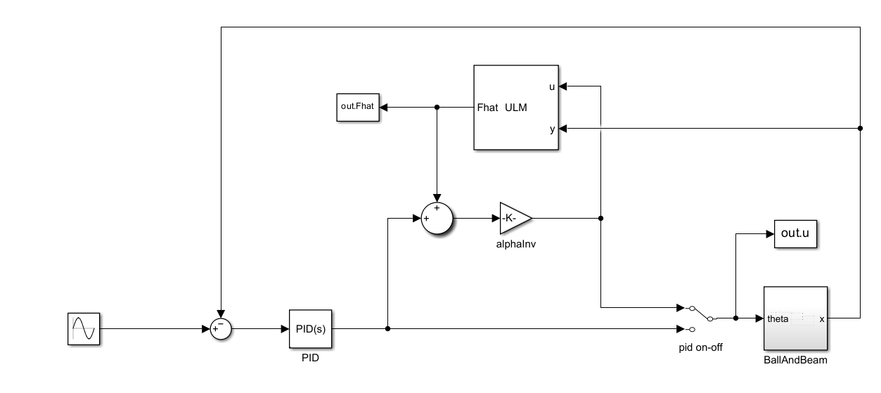
The intelligent PID has two main components to design. First you need a baseline PID controller, which you have already tuned as PID controller in the previous section and an Ultra-Local Model to estimate the plant uncertainties, which you will design in the next section. The overall control architecture for iPID implemented in Simulink is as follows,

Ultra-Local Model Design

The ULM block interface in Simulink has following tunable fields

• Input gain

• Model Order

• Sample time

• Integration Steps: is the discrete number of steps over which ULM model is estimated.

The tuned ULM parameters for the given example are as follows,

% Input Gain
% Set alpha = -0.225;
set_param([mdl, '/Ultra-Local Model'], 'alpha', '-0.225')

% Set the gain alphaInv to -1/alpha
set_param([mdl,'/alphaInv'], 'gain', '-1/(-0.225)')

Since Ball and Beam is a second-order system and we are using a PID as baseline controller, we will use Model Order for ULM block as '2' [1].

% Set the model Order
set_param([mdl, '/Ultra-Local Model'], 'modelOrder', '2')

% Set the ULM sample time
set_param([mdl, '/Ultra-Local Model'], 'Ts', '0.01')

% Integration window in number of discrete steps
set_param([mdl, '/Ultra-Local Model'], 'numIntegrationSteps', '1250')

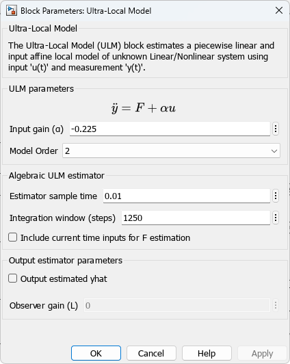
As aim of this example is closed-loop control of the given plant, we have no need for the output estimated 'yhat' and leave the option unchecked. However this additional output can be used to tune the ULM block or when ULM block is used as estimator (see Ultra-Local Model for System Identification and Output Prediction).

% Select the baseline PID controller
set_param([mdl,'/pid on-off'],'sw', useIntelligentPID)

% Simulate the model
out = sim(mdl);

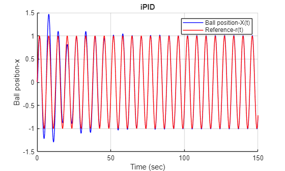
The iPID controller tracking performance

% Plot the simulation data
fig3 = figure();
hold on
grid on
plot(out.tout,out.y.Data,'b')
plot(out.tout,out.r.Data,'r')
xlabel('Time (sec)')
ylabel('Ball position-x')
legend('Ball position-X(t)','Reference-r(t)')
title('iPID')

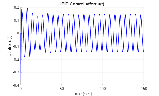
Plot total iPID control effort to track the reference command, and ULM estimate of the unmodeled plant dynamics

% Plot the control effort
fig4 = figure();
hold on
grid on
plot(out.tout,out.u.Data,'b')
xlabel('Time (sec)')
ylabel('Control u(t)')
title('iPID Control effort u(t)')

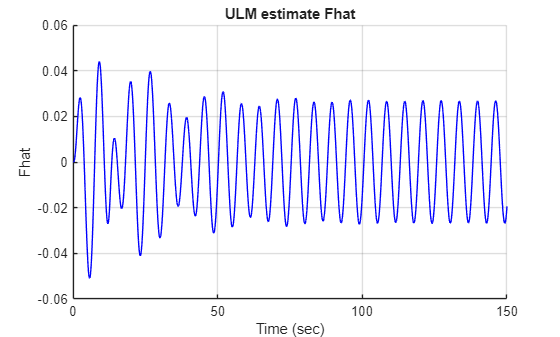
% ULM estimate of plant dynamics Fhat
fig5 = figure();
hold on
grid on
plot(out.tout,out.Fhat.Data,'b')
xlabel('Time (sec)')
ylabel('Fhat')
title('ULM estimate Fhat')

As seen from the above plots, iPID outperforms a fixed gain feedback controller in terms of tracking accuracy. This tracking improvement is due to controller actively canceling out local estimate of unmodeled dynamics of nonlinear plant and enforcing a second order double integrator error dynamics behavior.

% Close the model
close_system(mdl,0)

Conclusion

In this example we have demonstrated, how we can improve the performance of standard baseline controller by augmenting data driven techniques like ULM. This example demonstrates ULM estimates can be used by a fixed gain controller to actively mitigate uncertainties in the system. As demonstrated compared to a conventional PID controller, an ULM based Intelligent PID controller is able to provide a better tracking performance.

References

[1] Fliess, Michel, and Cédric Join. "Model-free control." International journal of control 86.12 (2013): 2228-2252.