Ultra-Local Model for System Identification and Output Prediction

This example show how to use the Ultra-Local Model (ULM) block in Simulink® for system identification and output prediction. The Ultra-Local Model block estimates a local linear control-affine model for a single-input single-output (SISO) plant at runtime. Popular applications of ULM include model-free control, where you augment a nominal controller with a ULM-based disturbance compensator, which is discussed in details in a separate example Intelligent PID using Ultra Local Model for Ball on Beam Balance. This example, however, serves as a tutorial on how ULM works and how to choose block parameters to obtain good identification and prediction results.

Ultra-Local Model Overview

The input-output behavior of a nonlinear SISO system is often described in the following generic form:

$${\mathit{y}}^{\left(\mathit{m}\right)}=\mathit{f}\left({\mathit{y}}^{\left(\mathit{m}-1\right)},\dots \mathit{y},{\mathit{u}}^{\left(\mathit{l}\right)},\dots \mathit{u}\right)$$.

Here, $\mathit{f}\left(.\right)$ is an unknown nonlinear function, $\mathit{y}$ is the plant output, $\mathit{u}$ is the plant input, $\mathit{m}$ is the m-th order derivative of plant output, and $\mathit{l}$ is the l-th order derivative of plant input.

The ULM method approximates the above plant using a simplified linear control-affine model as follows:

$${\mathit{y}}^{\left(\mathit{n}\right)}=\mathit{F}\left(\mathit{t}\right)+\alpha *\mathit{u}\left(\mathit{t}\right)$$,

Here,

• $\mathit{n}\in \left[1,2\right]$ is the order of ULM model. In practice, a first or second order ULM model is sufficient to describe the plant local behavior.

• $\mathit{F}\left(\mathit{t}\right)\in \mathit{R}$subsumes unmodeled dynamics and/or external disturbances. Therefore, $\mathit{F}\left(\mathit{t}\right)$must be continuously updated at runtime to approximate the local plant behavior.

• $\alpha \in \mathit{R}$ is the input gain and is chosen such that the three quantities ${\mathit{y}}^{\left(\mathit{n}\right)}$, $\mathit{F}\left(\mathit{t}\right)$, and $\alpha *\mathit{u}\left(\mathit{t}\right)$ are of the same order of magnitude. $\alpha$is usually a constant and it does not have to be precise.

In other words, the ULM model approximates the local behavior of a nonlinear plant as a single or double integrator plus a time-varying quantity $\mathit{F}\left(\mathit{t}\right)$that captures local uncertainties and disturbances. The ULM block can identify $\mathit{F}\left(\mathit{t}\right)$ from the plant input and output data online, using first-order or second order Algebraic Estimation methods (see Ultra-Local Model for Disturbance Estimation and Compensation).

Online Identification of First-Order Ultra-Local Model

This section shows how to use the ULM block to estimate $\mathit{F}\left(\mathit{t}\right)$ for a first-order ULM model.

Ground Truth

For the sake of simplification, the true plant used in this tutorial is a linear system:

$$\dot{\mathit{y}}=\left(\mathit{t}+3\right)+2\mathit{u}$$

Because the plant shares the same structure as the first-order ULM model, such as

• Model order n = 1

• Time-varying quantity $\mathit{F}\left(\mathit{t}\right)=\mathit{t}+3$

• The input gain $\alpha =2$

This example demonstrates ULM block does a good job estimating $\mathit{F}\left(\mathit{t}\right)$.

Connect Ultra-Local Model Block

To examine how the ULM block is connected to the plant for online identification, open the Simulink model ulmFirstOrder.slx that estimates the first-order ULM.

mdl = 'ulmFirstOrder';
ulm_block = [mdl '/Ultra-Local Model'];
open_system(mdl);

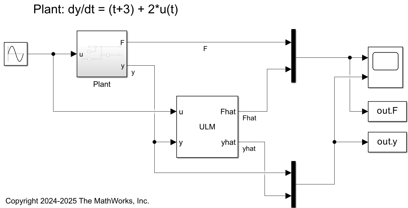
ULM block takes measured plant input and output signals as inputs and produces $\hat{\mathit{F}}$ and $\hat{\mathit{y}}$, which is a one-step prediction of plant output $\hat{\mathit{y}}\left(\mathit{t}+\mathrm{Ts}\right)$. In this example, you use sine wave as input signal but it can be other types of excitation signals as well, such as step or random perturbation.

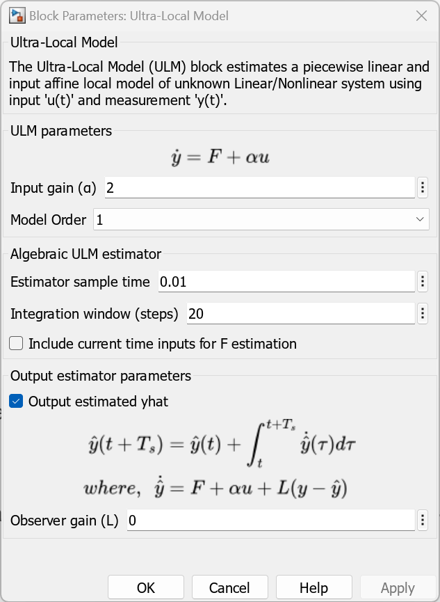
ULM Block Parameters

This section discusses some guidelines regarding how to tune the ULM block parameters and achieve good estimation of $\hat{\mathit{F}}$. There are four main design parameters: model order, input gain, estimator sample time, and integration window (steps).

Model Order (n)

Generally, the ULM model order can be less than or equal to the true plant order such that $\mathit{n}\le \mathit{m}$. In practice, using first or second order ULM model is often sufficient to approximate local behavior. In this tutorial, choose $\mathit{n}=1$ because the true plant order is 1.

In addition, when ULM is used as a part of model-free control structure to provide disturbance compensation, the choice of ULM model order also depends on choice of the nominal controller. For example, if the nominal control law is proportional-only (P) or proportional-integral (PI), ULM model order $\mathit{n}=1$ is sufficient. However, if the nominal control law is proportional-derivative (PD) or proportional-integral-derivative (PID), ULM model order of $\mathit{n}=2$ is required.

Input Gain ($\alpha$)

A precise guess for input gain $\alpha$is not strictly required for ULM to work. Generally speaking the choice of $\alpha \in {\mathit{R}}^{+}$ is required to approximately balance the three quantities $\dot{\mathit{y}}$, $\mathit{F}\left(\mathit{t}\right)$, and $\alpha *\mathit{u}\left(\mathit{t}\right)$ in their magnitude. Any mismatch between $\alpha$ and the true value in the plant is more or less captured by $\hat{\mathit{F}}$.

In addition, the definition of $\alpha$is the same as the critical gain ${\mathit{b}}_0$used in the Active Disturbance Rejection Control (ADRC) block. For recommendations how to obtain good initial guess of this parameter, see Ultra-Local Model for Disturbance Estimation and Compensation.

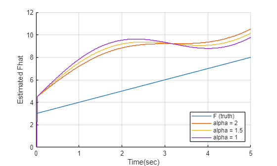
Examine the impact of input gain $\alpha$on the estimation results.

% Set the "alpha" parameter the same as the ground truth value
set_param(ulm_block,'alpha','2');
% simulate
out1 = sim(mdl);
% Set the "alpha" parameter with a small difference from the truth
set_param(ulm_block,'alpha','1.5');
% simulate
out2 = sim(mdl);
% Set the "alpha" parameter with a large difference from the truth
set_param(ulm_block,'alpha','1');
% simulate
out3 = sim(mdl);
% plot ground truth
figure;
hold on;
grid on
plot(out1.F);
% plot estimated Fhat
plot(out1.Fhat);
plot(out2.Fhat);
plot(out3.Fhat);
% legend
xlabel('Time(sec)')
ylabel('Estimated Fhat')
legend({'F (truth)','alpha = 2','alpha = 1.5','alpha = 1'},'Location','southeast');

% reset alpha to truth
set_param(ulm_block,'alpha','2');

As expected, the deviation of $\hat{\mathit{F}}$ from the true $\mathit{F}$ increases when input gain $\alpha$becomes further away from the truth. The periodical fluctuation in $\hat{\mathit{F}}$comes from $\left(\alpha -2\right)*\mathit{u}\left(\mathit{t}\right)$ as the excitation signal $\mathit{u}\left(\mathit{t}\right)$ is a sine wave.

Estimator Sample Time (${\mathit{T}}_{\mathit{S}}$)

Estimator sample time ${\mathit{T}}_{\mathit{S}}$ is the sample time at which ULM updates estimation of $\hat{\mathit{F}}$. Faster sample time means that the collected run-time data used for estimation are closer to the local operating condition, which in turn improves estimation accuracy. Since $\hat{\mathit{F}}$ from ULM is often used as part of control law, ULM only needs to run as fast as the controller demands.

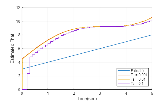
Examine the impact of the estimator sample time ${\mathit{T}}_{\mathit{S}}$ on the estimation results.

% Set fast sample time
set_param(ulm_block,'Ts','0.001');
% simulate
out1 = sim(mdl);
% Set medium sample time
set_param(ulm_block,'Ts','0.01');
% simulate
out2 = sim(mdl);
% Set slow sample time
set_param(ulm_block,'Ts','0.1');
% simulate
out3 = sim(mdl);
% plot ground truth
figure;
hold on
grid on
plot(out1.F);
% plot estimated Fhat
plot(out1.Fhat);
plot(out2.Fhat);
plot(out3.Fhat);
% legend
xlabel('Time(sec)')
ylabel('Estimated Fhat')
legend({'F (truth)','Ts = 0.001','Ts = 0.01','Ts = 0.1'},'Location','southeast');

% reset Ts
set_param(ulm_block,'Ts','0.01');

As expected, the deviation of $\hat{\mathit{F}}$ from the true $\mathit{F}$ increases when Estimator sample time ${\mathit{T}}_{\mathit{S}}$ becomes slower.

Integration Window (steps)

$\hat{\mathit{F}}$ is estimated using an algebraic estimation algorithm. The algorithm collects the plant input and output signals during an integration window from time $\mathit{t}-\mathit{N}*{\mathit{T}}_{\mathit{S}}$ to current time $\mathit{t}$ to compute $\hat{\mathit{F}}$. $\mathit{N}$ is the integration window that you can specify in the ULM block. The block requires parameter $\mathit{N}\ge 3$ to work properly. Generally, $\mathit{N}$cannot be too small because a small $\mathit{N}$ would reduce numerical integration accuracy as well as robustness toward the measurement noise. $\mathit{N}$cannot be too large either because a large $\mathit{N}$ uses more historical data that might prevent $\hat{\mathit{F}}$ from accurately reflecting the local plant behavior.

Examine the impact of the integration window steps $\mathit{N}$ on the estimation results.

% Set a small integration window
set_param(ulm_block,'numIntegrationSteps','5');
% simulate
out1 = sim(mdl);
% Set a medium integration window
set_param(ulm_block,'numIntegrationSteps','20');
% simulate
out2 = sim(mdl);
% Set a large integration window
set_param(ulm_block,'numIntegrationSteps','50');
% simulate
out3 = sim(mdl);
% plot ground truth
figure
hold on
grid on
plot(out1.F);
% plot estimated Fhat
plot(out1.Fhat);
plot(out2.Fhat);
plot(out3.Fhat);
% legend
xlabel('Time(sec)')
ylabel('Estimated Fhat')
legend({'F (truth)','N = 5','N = 20','N = 50'},'Location','southeast');

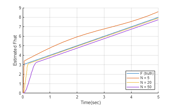
% reset N
set_param(ulm_block,'numIntegrationSteps','20');

As expected, $\mathit{N}=20$ gives the best estimation result as it balances between numerical accuracy and local behavior.

One-Step Prediction

In addition to $\hat{\mathit{F}}$, ULM block also produces $\hat{\mathit{y}}$, the one-step prediction of plant output $\mathit{y}$ at time $\mathit{t}+{\mathit{T}}_{\mathit{S}}$ based on the estimated $\hat{\mathit{F}}$. You can enable the optional outport yhat in the ULM block using the Output estimated yhat option in the block parameters. Typically, $\hat{\mathit{y}}$ is helpful in one of the following two ways.

Use $\hat{\mathit{y}}$ to Check Accuracy of $\hat{\mathit{F}}$

By comparing $\hat{\mathit{y}}$ with measured$\mathit{y}$, you can tell how well $\hat{\mathit{F}}$ is estimated by the ULM block. This is very useful because you usually don't know the ground truth of $\mathit{F}$ in practice.

Examine the impact of the integration window steps $\mathit{N}$ on the estimation results by looking at $\hat{\mathit{y}}$.

% plot ground truth
figure();hold on;grid on
plot(out1.y);
% plot estimated Fhat
plot(out1.yhat);
plot(out2.yhat);
plot(out3.yhat);
% legend
xlabel('Time(sec)')
ylabel('One-Step Estimation (yhat)')
legend({'y (truth)','N = 5','N = 20','N = 50'},'Location','southeast');

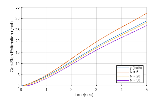
It is clear that $\mathit{N}=20$ produces the best prediction result among the three values as we already know from the previous analysis when ground truth of $\mathit{F}$ is known.

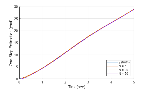
Use $\hat{\mathit{y}}$ for One-Step Prediction

Some control laws require one-step prediction and the $\hat{\mathit{y}}$ port in the ULM block can provide such information. To predict it accurately, however, you need to enable the Luenberger observer by specifying the observer gain $\mathit{L}\ge 0$ in the ULM block dialog.

% enable Luenberger observer by specifying observer gain L
set_param(ulm_block,'ObsvGain','5');
% Set a small integration window
set_param(ulm_block,'numIntegrationSteps','5');
% simulate
out1 = sim(mdl);
% Set a medium integration window
set_param(ulm_block,'numIntegrationSteps','20');
% simulate
out2 = sim(mdl);
% Set a large integration window
set_param(ulm_block,'numIntegrationSteps','50');
% simulate
out3 = sim(mdl);
% plot ground truth
figure();hold on;grid on
plot(out1.y);
% plot estimated Fhat
plot(out1.yhat);
plot(out2.yhat);
plot(out3.yhat);
% legend
xlabel('Time(sec)')
ylabel('One-Step Estimation (yhat)')
legend({'y (truth)','N = 5','N = 20','N = 50'},'Location','southeast');

% reset N
set_param(ulm_block,'numIntegrationSteps','20');

Compared to the previous plot, the the Luenberger observer improves one-step prediction in all the three cases.

% Close the model
close_system(mdl,0);

Online Identification of Second-Order Ultra-Local Model

This section shows how to use ULM block to estimate $\mathit{F}\left(\mathit{t}\right)$ for a second-order ULM model.

Ground Truth

Consider a second-order linear system as follows:

$$\ddot{\mathit{y}}=\left(\mathit{t}+3\right)+2\mathit{u}$$

The plant shares the same structure as the first-order ULM model, such as

• Model order n = 2

• Time-varying quantity $\mathit{F}\left(\mathit{t}\right)=\mathit{t}+3$

• The input gain $\alpha =2$

Simulation and Results

To tune the parameters, you can use the recommendations from the preceding sections. Open the Simulink model that estimates the second-order ULM.

mdl = 'ulmSecondOrder';
ulm_block = [mdl '/Ultra-Local Model'];
open_system(mdl);

The ideal value for input-gain is $\alpha =2$.

%set the parameter alpha to true value
set_param(ulm_block,'alpha','2');

Model order second-order ULM case is known and set to 2. The best performing sample time and integration window is $\mathit{Ts}$ = 0.01 and $\mathit{N}$ = 85.

% Set medium sample time
set_param(ulm_block,'Ts','0.01');

% Set a small integration window
set_param(ulm_block,'numIntegrationSteps','85');

Similar to first-order case, you can use the ULM block as one step predictor for second-order case. Enable the Luenberger observer and specify the observer gain $\mathit{L}\ge 0$ in the ULM block parameters.

% enable Luenberger observer by specifying observer gain L
set_param(ulm_block,'ObsvGain','5');

With all parameters defined, simulate the model and plot the results.

% simulate
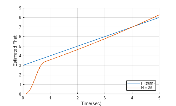
out = sim(mdl);

Plot ULM model estimate $\mathit{F}\mathrm{vs}\hat{\mathit{F}}$.

% plot ground truth
figure();hold on;grid on
plot(out.F);
% plot estimated Fhat
plot(out.Fhat);
% legend
xlabel('Time(sec)')
ylabel('Estimated Fhat')
legend({'F (truth)','N = 85'},'Location','southeast');

Plot the estimator output $\mathit{y}\mathrm{vs}\hat{\mathit{y}}$ for second-order case.

% plot ground truth
figure();hold on;grid on
plot(out.y);
% plot estimated yhat
plot(out.yhat);
% legend
xlabel('Time(sec)')
ylabel('One-Step Estimation (yhat)')
legend({'y (truth)','N = 100 & L = 5'},'Location','southeast');

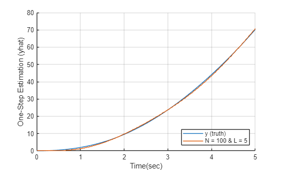
Similar to first-order case, the Luenberger observer improves one-step prediction.

% Close the model
close_system(mdl,0);

References

[1] Fliess, Michel, and Cédric Join. "Model-free control." International journal of control 86.12 (2013): 2228-2252.