Ultra-Local Model

Estimate nonlinear plant as single or double integrator systems with an affine term that captures unknown dynamics and disturbances

Since R2025a

• 

Libraries:
Simulink Control Design / Disturbance Observer

Description

Ultra-local model (ULM) is an estimation technique that allows you to approximate a nonlinear plant as a single or double integrator system with an affine term that captures unknown dynamics and disturbances. The estimated model is valid only for a local operating point over a short period of time. You can the Ultra-Local Model block for ULM-based estimation. Using this block, you can estimate first-order and second-order local plant dynamics of the following form:

• First order — $$\dot{y}=F+\alpha u$$

• Second-order — $$\ddot{y}=F+\alpha u$$

Here, α is the input gain for tuning and F is the affine term for combined uncertain dynamics and external disturbances.

You can use this block either as a standalone estimator for disturbance estimation and output prediction or use its disturbance estimation capabilities for improving nominal controller performance.

For more information about ULM-based estimation, see Ultra-Local Model for Disturbance Estimation and Compensation.

Examples

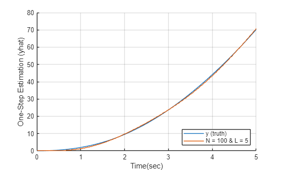
Ultra-Local Model for System Identification and Output Prediction

Use the Ultra-Local Model block for system identification and output prediction.

• Open Live Script

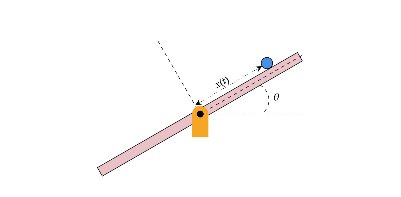
Intelligent PID using Ultra Local Model for Ball on Beam Balance

Implement model-free intelligent PID control technique using ultra-local model.

• Open Live Script

Ports

Input

u — Plant input

scalar

Specify the plant input at this port.

Data Types: single | double

y — Plant output

scalar

Specify the measured plant output at this port.

Data Types: single | double

Output

Fhat — Estimated disturbances and unmodeled dynamics

scalar

Estimated disturbances in the model. The block calculates these disturbances over a small integration window using algebraic estimation methods. These disturbances can include both unmodeled dynamics and external disturbances.

Data Types: single | double

yhat — Estimated output

scalar

One-step prediction of the plant output y at time t+Ts based on the estimated $$\widehat{F}$$.

Dependencies

To enable this port, select Output estimated yhat.

Data Types: single | double

Parameters

To edit block parameters interactively, use the Property Inspector. From the Simulink^® Toolstrip, on the Simulation tab, in the Prepare gallery, select Property Inspector.

Input gain (α) — Input gain

1 (default) | nonzero finite scalar

Input gain, specified as a nonzero finite scalar value. For ULM to work, you do not require a precise guess for input gain α. The block requires you to select an α ∈ R to approximately balance the three quantities y⁽ⁿ⁾, F(t), and αu(t) in their magnitude. The estimated $$\widehat{F}$$ captures any mismatch between α and the true plant value.

Programmatic Use

To set the block parameter value programmatically, use the set_param function.

Parameter:	alpha
Values:	"1" (default) | nonzero finite scalar in quotes

Example: set_param(gcb,"alpha","2");

Model Order — Ultra-local model order

1 (default) | 2

Order of the ultra local model, specified as a first-order or second-order model.

• First order — $$\dot{y}=F+\alpha u$$

• Second-order — $$\ddot{y}=F+\alpha u$$

Generally, the ULM model order can be less than or equal to the true plant order. In addition, when you use ULM as a part of model-free control structure to provide disturbance compensation, the choice of ULM model order also depends on choice of the nominal controller. For example, if the nominal control law is proportional-only (P) or proportional-integral (PI), first-order ULM is sufficient. However, if the nominal control law is proportional-derivative (PD) or proportional-integral-derivative (PID), you require a second-order ULM.

Programmatic Use

To set the block parameter value programmatically, use the set_param function.

Parameter:	modelOrder
Values:	"1" (default) | "2"

Example: set_param(gcb,"modelOrder","2");

Estimator sample time — Estimator sample time

0.01 (default)

The estimator sample time Ts is the time at which the ULM updates its estimation of $$\widehat{F}$$. A faster sample time means that the collected runtime data used for estimation is closer to the local operating condition, which, in turn, improves estimation accuracy. Since, typical applications of ULM often involve using $$\widehat{F}$$ as part of the control law, it only needs to run as fast as the controller demands.

Programmatic Use

To set the block parameter value programmatically, use the set_param function.

Parameter:	Ts
Values:	"0.01" (default) | positive scalar in quotes

Example: set_param(gcb,"Ts","0.02");

Integration window (steps) — Integration window

3 (default) | positive integer greater than 3

Integration window, specified as a positive integer greater than 3. The block estimates F(t) using an algebraic estimation algorithm. To compute $$\widehat{F}$$, the algorithm collects the plant input and output signals during an integration window, from time t − N×Ts to current time t. Here, N is the integration window that you can specify in the ULM block. The block requires the parameter N to be at least 3 to function properly. Generally, N cannot be too small because a small N would reduce numerical integration accuracy and robustness against measurement noise. Conversely, N cannot be too large because a large N uses more historical data, which might prevent $$\widehat{F}$$ from accurately reflecting the local plant behavior.

Programmatic Use

To set the block parameter value programmatically, use the set_param function.

Parameter:	numIntegrationSteps
Values:	"3" (default) | positive integer greater than 3 in quotes

Example: set_param(gcb,"numIntegrationSteps","5");

Include current time inputs for F estimation — Include current time inputs for estimation

off (default) | on

Flag to include current plant input and output steps for estimating F.

• off — Use only the previous N steps of plant data u(t) and y(t) for estimating F, where N is the integration window.

• on — Include the data from current time step of u(t) and y(t) for estimating F. The integration window size then becomes N+1.

Programmatic Use

To set the block parameter value programmatically, use the set_param function.

Parameter:	useCurrentdata
Values:	"off" (default) | "on"

Example: set_param(gcb,"useCurrentdata","on");

Output estimated yhat — Output one-step estimation of output

off (default) | on

Enable this option to return the one-step prediction of the plant output y at time t+Ts based on the estimated $$\widehat{F}$$ at the output port yhat. The block computes this as follows:

• First order — $$\begin{array}{l}\widehat{y}(t+T_s)=\widehat{y}(t)+{\displaystyle {\int }_t^{t+T_s}\dot{\widehat{y}}(\tau )d\tau },\\ \dot{\widehat{y}}=\widehat{F}+\alpha u+L(y-\widehat{y})\end{array}$$

• Second order — $$\begin{array}{l}\widehat{y}(t+T_s)=\widehat{y}(t)+{\displaystyle \int {\displaystyle {\int }_t^{t+T_s}\ddot{\widehat{y}}(\tau )d\tau }},\\ \ddot{\widehat{y}}=\widehat{F}+\alpha u+L(y-\widehat{y})\end{array}$$

Programmatic Use

To set the block parameter value programmatically, use the set_param function.

Parameter:	enableYhatport
Values:	"off" (default) | "on"

Example: set_param(gcb,"enableYhatport","on");

Observer gain (L) — Observer gain

0 (default) | nonnegative scalar

Observer gain, specified as a nonnegative scalar. Specifying an observer gain helps produce more accurate estimations of yhat.

Dependencies

To enable this options, select Output estimated yhat.

Programmatic Use

To set the block parameter value programmatically, use the set_param function.

Parameter:	ObsvGain
Values:	"0" (default) | nonnegative scalar in quotes

Example: set_param(gcb,"ObsvGain","2");

Extended Capabilities

C/C++ Code Generation
Generate C and C++ code using Simulink® Coder™.

Version History

Introduced in R2025a