Main Content

Nonlinear Inductor

Inductor with nonideal core

  • Nonlinear Inductor block

Libraries:
Simscape / Electrical / Passive

Description

The Nonlinear Inductor block represents an inductor with a nonideal core. A core may be nonideal due to its magnetic properties and dimensions. To choose between these parameterization options, use the Parameterized by parameter:

Single Inductance (Linear)

These equations define the relationships between voltage, current, and flux,

i=iL+vGp

v=NwdΦdt

Φ=LNwiL

where:

  • v is the terminal voltage.

  • i is the terminal current.

  • iL is the current through inductor.

  • Gp is the parasitic parallel conductance.

  • Nw is the number of winding turns.

  • Φ is the magnetic flux.

  • L is the unsaturated inductance.

Single Saturation Point

These equations define the relationships between voltage, current, and flux,

i=iL+vGp

v=NwdΦdt

Φ=LNwiL (for unsaturated)

Φ=LsatNwiL±Φoffset (for saturated)

where:

  • v is the terminal voltage.

  • i is the terminal current.

  • iL is the current through inductor.

  • Gp is the parasitic parallel conductance.

  • Nw is the number of winding turns.

  • Φ is the magnetic flux.

  • Φoffset is the magnetic flux saturation offset.

  • L is the unsaturated inductance.

  • Lsat is the saturated inductance.

Magnetic Flux Versus Current Characteristic

These equations define the relationships between voltage, current, and flux,

i=iL+vGp

v=NwdΦdt

Φ=f(iL)

where:

  • v is the terminal voltage.

  • i is the terminal current.

  • iL is the current through inductor.

  • Gp is the parasitic parallel conductance.

  • Nw is the number of winding turns.

  • Φ is the magnetic flux.

The block determines magnetic flux by using a one-dimensional table lookup, based on the vector of electrical current values and the vector of corresponding magnetic flux values that you provide. You can construct these vectors using negative and positive data, or positive data only. If you use positive data only, the first element of the vector must be 0. The block calculates negative values by rotating the positive data by 180° about (0,0).

Magnetic Flux Density Versus Magnetic Field Strength Characteristic

These equations define the relationships between voltage, current, and flux,

i=iL+vGp

v=NwdΦdt

Φ=BAe

B=f(H)

H=NwleiL

where:

  • v is the terminal voltage.

  • i is the terminal current.

  • iL is the current through inductor.

  • Gp is the parasitic parallel conductance.

  • Nw is the number of winding turns.

  • Φ is the magnetic flux.

  • B is the magnetic flux density.

  • H is the magnetic field strength.

  • le is the effective core length.

  • Ae is the effective core cross-sectional area.

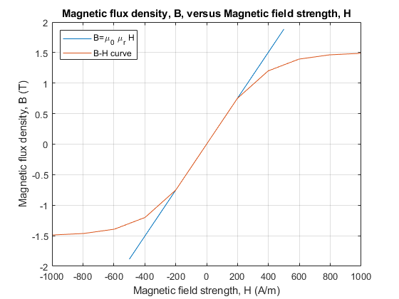
The block determines the magnetic flux density by one-dimensional table lookup, based on the vector of magnetic field strength values and the vector of corresponding magnetic flux density values that you provide. You can construct these vectors using either negative and positive data, or positive data only. If you use positive data only, the first element of the vector must be 0. The block calculates negative values by rotating the positive data by 180° about (0,0).

Magnetic Flux Density Versus Magnetic Field Strength Characteristic with Hysteresis

These equations define the relationships between voltage, current, and flux,

i=iL+vGp

v=NwdΦdt

Φ=BAe

B=μ0(H+M)

H=NwleiL

where:

  • v is the terminal voltage.

  • i is the terminal current.

  • iL is the current through inductor.

  • Gp is the parasitic parallel conductance.

  • Nw is the number of winding turns.

  • Φ is the magnetic flux.

  • B is the magnetic flux density.

  • μ0 is the magnetic permeability of a vacuum.

  • H is the magnetic field strength.

  • M is the magnetization of the inductor core.

  • le is the effective core length.

  • Ae is the effective core cross-sectional area.

The magnetization acts to increase the magnetic flux density, and its value depends on both the current value and the history of the field strength. The block uses the Jiles-Atherton 1, 2] equations to determine M at any given time. This figure shows a typical plot of the resulting relationship between B and H.
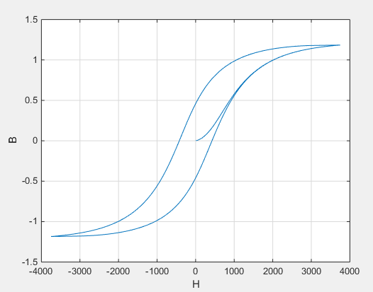
As the field strength increases from H = 0, the plot initially follows an ascending hysteresis curve. At the saturation point, further increases in field intensity no longer cause significant increases in magnetic flux.

As you reduce the magnetic field strength from the saturation point, the plot follows a descending hysteresis curve. The difference between ascending and descending curves is due to the dependence of M on the trajectory history. Physically, the behavior corresponds to magnetic dipoles in the core aligning as the field strength increases, but not then fully recovering to their original position as field strength decreases.

The starting point for the Jiles-Atherton equation is the split of the magnetization effect into two parts, one part that is purely a function of effective field strength Heff and another, irreversible part that depends on history. This equation defines the relative contributions of the anhysteretic magnetisation Man and the irreversible magnetization Mirr to the total magnetization M,

M=cMan+(1c)Mirr,

where c is the coefficient for reversible magnetization.

This equation relates Man to the equivalent magnetizationHeff:

Man=Ms(coth(Heffa)aHeff).

The function defines a saturation curve with limiting values ±Ms, where:

  • Ms is the saturation magnetization.

  • a is the anhysteretic magnetization coefficient, which determines the point of saturation. It approximately describes the average of the two hysteretic curves.

In the Nonlinear Inductor block mask, you provide values for dMan/dHeff when Heff = 0 and a point [H1, B1] on the anhysteretic B-H curve. The block uses these values to determine values for a and Ms.

The Jiles-Atherton model defines the irreversible term by a partial derivative with respect to field strength,

dMirrdH=ManMirrKδα(ManMirr)δ={1if H01if H<0 

where:

  • K is the bulk coupling coefficient, which shapes the irreversible characteristic.

  • α is the inter-domain coupling factor.

Comparison of the equation with a standard first-order differential equation reveals that as you change the total field strength H, the irreversible term Mirr attempts to track the reversible term Man, but with a variable tracking gain of 1/(Kδα(ManMirr)). The tracking error acts to create the hysteresis at the points where δ changes sign.

This equation defines the effective field strength of an anhysteretic curve,

Heff=H+αM.

The value of α affects the shape of the hysteresis curve. Larger values act to increase the B-axis intercepts. However, the stability term Kδα(ManMirr) must be positive for δ > 0 and negative for δ < 0. There are therefore limits on the values of α that you can provide. A typical maximum value is of the order 1e-3.

Procedure for Finding Approximate Values for Jiles-Atherton (JA) Equation Coefficients

You can determine representative values for the equation coefficients using this procedure:

  1. Provide a value for the Anhysteretic B-H gradient when H is zero parameter (dMan/dHeff when Heff = 0) and a data point [H1, B1] on the anhysteretic B-H curve. From these values, the block initialization determines values for α and Ms.

  2. Set the Coefficient for reversible magnetization, c parameter to achieve correct initial B-H gradient when starting a simulation from [H B] = [0 0]. The value of c is approximately the ratio of this initial gradient to the Anhysteretic B-H gradient when H is zero. The value of c must be greater than 0 and less than 1.

  3. Set the Bulk coupling coefficient, K parameter to the approximate magnitude of H when B = 0 on the ascending hysteresis curve.

  4. Start with a very small value for the Inter-domain coupling factor, alpha parameter, and gradually increase it to tune the value of B when crossing the H = 0 line. A typical value is in the range of 1e-4 to 1e-3. Values that are too large cause the gradient of the B-H curve to tend to infinity, which is nonphysical and generates a run-time assertion error.

To get a good match against a predefined B-H curve, iterate on these four steps.

Examples

Ports

Conserving

expand all

Electrical conserving port associated with the positive terminal.

Electrical conserving port associated with the negative terminal.

Parameters

expand all

Main

Parameterization method that you use to describe the B-H curve. Choose one of these options:

  • Single inductance (linear) — Provide the values for number of turns, unsaturated inductance, and parasitic parallel conductance.

  • Single saturation point — Provide the values for number of turns, unsaturated and saturated inductances, saturation magnetic flux, and parasitic parallel conductance.

  • Magnetic flux versus current characteristic — In addition to the number of turns and the parasitic parallel conductance value, provide the current vector and the magnetic flux vector, to populate the magnetic flux versus current lookup table.

  • Magnetic flux density versus magnetic field strength characteristic — In addition to the number of turns and the parasitic parallel conductance value, provide the values for effective core length and cross-sectional area, as well as the magnetic field strength vector and the magnetic flux density vector, to populate the magnetic flux density versus magnetic field strength lookup table.

  • Magnetic flux density versus magnetic field strength characteristic with hysteresis — In addition to the number of turns and the effective core length and cross-sectional area, provide the values for the initial anhysteretic B-H curve gradient, the magnetic flux density and field strength at a certain point on the B-H curve, as well as the coefficient for the reversible magnetization, bulk coupling coefficient, and inter-domain coupling factor, to define magnetic flux density as a function of both the current value and the history of the field strength.

Total number of turns of wire wound around the inductor core.

Inductance when the inductor operates in its linear region.

Dependencies

To enable this parameter, set Parameterized by to Single inductance (linear) or Single saturation point.

Inductance when the inductor operates beyond its saturation point.

Dependencies

To enable this parameter, set Parameterized by to Single saturation point.

Magnetic flux at which the inductor saturates.

Dependencies

To enable this parameter, set Parameterized by to Single saturation point.

Current data that the block uses to populate the magnetic flux versus current lookup table.

Dependencies

To enable this parameter, set Parameterized by to Magnetic flux versus current characteristic.

Magnetic flux data that the block uses to populate the magnetic flux versus current lookup table.

Dependencies

To enable this parameter, set Parameterized by to Magnetic flux versus current characteristic.

Magnetic field intensity H, specified as a vector with the same number of elements as the magnetic flux density vector B.

Dependencies

To enable this parameter, set Parameterized by to Magnetic flux density versus magnetic field strength characteristic.

Magnetic flux density B, specified as a vector with the same number of elements as the magnetic field strength vector H.

Dependencies

To enable this parameter, set Parameterized by to Magnetic flux density versus magnetic field strength characteristic.

Effective core length. This parameter represents the average length of the magnetic path around the core.

Dependencies

To enable this parameter, set Parameterized by to Magnetic flux density versus magnetic field strength characteristic or Magnetic flux density versus magnetic field strength characteristic with hysteresis.

Effective core cross-sectional area. This parameter represents the average area of the magnetic path around the core.

Dependencies

To enable this parameter, set Parameterized by to Magnetic flux density versus magnetic field strength characteristic or Magnetic flux density versus magnetic field strength characteristic with hysteresis.

Gradient of the anhysteretic B-H curve around zero field strength. Set this parameter to the average gradient of the ascending and descending hysteresis curves.

Dependencies

To enable this parameter, set Parameterized by to Magnetic flux density versus magnetic field strength characteristic with hysteresis.

Flux density of the point for field strength measurement. You must specify a point on the anhysteretic curve by providing its flux density value. To obtain accurate results, pick a point at high field strength where the ascending and descending hysteresis curves align.

Dependencies

To enable this parameter, set Parameterized by to Magnetic flux density versus magnetic field strength characteristic with hysteresis.

Field strength that corresponds to the point that you define by the Flux density point on anhysteretic B-H curve parameter.

Dependencies

To enable this parameter, set Parameterized by to Magnetic flux density versus magnetic field strength characteristic with hysteresis.

Coefficient for reversible magnetization in the Jiles-Atherton equations, c. This parameter represents the proportion of the magnetization that you can reverse.

Dependencies

To enable this parameter, set Parameterized by to Magnetic flux density versus magnetic field strength characteristic with hysteresis.

Bulk coupling coefficient in the Jiles-Atherton equations, K. This parameter primarily controls the field strength magnitude at which the B-H curve crosses the zero flux density line.

Dependencies

To enable this parameter, set Parameterized by to Magnetic flux density versus magnetic field strength characteristic with hysteresis.

Inter-domain coupling factor in the Jiles-Atherton equations, α. This parameter primarily affects the points at which the B-H curves intersect the zero field strength line. Typical values are in the range of 1e-4 to 1e-3.

Dependencies

To enable this parameter, set Parameterized by to Magnetic flux density versus magnetic field strength characteristic with hysteresis.

Averaging period for the hysteresis losses calculation. These losses are proportional to the area enclosed by the B-H trajectory. If you excite the block at a known, fixed frequency, you can set this value to the corresponding excitation period to calculate the hysteresis loss. The block logs the hysteresis loss once per AC cycle in the power_dissipated variable in the logged simulation data. If you are using a fixed-step solver, this value must be an integer multiple of the simulation step size.

If you do not excite the block at a known, fixed frequency, set this parameter to 0. The block sets the power_dissipated variable in the logged simulation data to 0. You can calculate the actual hysteresis loss by post-processing the power_instantaneous variable in the logged simulation data.

Dependencies

To enable this parameter, set Parameterized by to Magnetic flux density versus magnetic field strength characteristic with hysteresis.

Parasitic parallel conductance. Use this parameter to represent small parasitic effects. For some circuit topologies, you need a small parallel conductance.

Lookup table interpolation option. Select one of the following interpolation methods:

  • Linear — Select this option to get the best performance.

  • Smooth — Select this option to produce a continuous curve with continuous first-order derivatives.

For more information about interpolation algorithms, see the PS Lookup Table (1D) block reference page.

Dependencies

To enable this parameter, set Parameterized by to Magnetic flux versus current characteristic or Magnetic flux density versus magnetic field strength characteristic.

Initial Conditions

Initial state specification. Choose one of these options:

  • Current — Specify the initial state of the inductor by the initial current through the inductor iL.

  • Magnetic flux — Specify the initial state of the inductor by the magnetic flux.

Dependencies

To enable this parameter, in the Main settings, set the Parameterized by parameter to one of these options:

  • Single inductance (linear)

  • Single saturation point

  • Magnetic flux versus current characteristic

  • Magnetic flux density versus magnetic field strength characteristic

Initial current value that the block uses to calculate the value of magnetic flux at time zero. This parameter is the current passing through the inductor. Component current consists of current passing through the inductor and current passing through the parasitic parallel conductance.

Dependencies

To enable this parameter, set Specify initial state by to Current.

Magnetic flux at time zero.

Dependencies

To enable this parameter, set Specify initial state by to Magnetic flux.

Magnetic flux density at time zero.

Dependencies

To enable this parameter, in the Main settings, set the Parameterized by parameter to Magnetic flux density versus magnetic field strength characteristic with hysteresis.

Magnetic field strength at time zero.

Dependencies

To enable this parameter, in the Main settings, set the Parameterized by parameter to Magnetic flux density versus magnetic field strength characteristic with hysteresis.

References

[1] Jiles, D. C. and D. L. Atherton. "Theory of ferromagnetic hysteresis." Journal of Magnetism and Magnetic Materials 61, no. 1–2 (September 1986): 48–60.https://doi.org/10.1016/0304-8853(86)90066-1.

[2] Jiles, D. C. and D. L. Atherton. “Ferromagnetic hysteresis.” IEEE® Transactions on Magnetics 19, no. 5 (September 1983): 2183–2185. https://doi.org/10.1109/TMAG.1983.1062594.

Extended Capabilities

C/C++ Code Generation
Generate C and C++ code using Simulink® Coder™.

Version History

Introduced in R2012b
Go to top of page