Choose Classifier Options in Classification Learner
Choose Classifier Type
You can use Classification Learner to automatically train a selection of different classification models on your data. Use automated training to quickly try a selection of model types, then explore promising models interactively. To get started, try these options first:

| Get Started Classifier Options | Description |
|---|---|
| All Quick-To-Train | Try this option first. The app will train all the model types available for your data set that are typically fast to fit. |
| All Linear | Try this option if you expect linear boundaries between the classes in your data. This option fits only linear SVM, efficient linear SVM, efficient logistic regression, and linear discriminant models. The option also fits a binary GLM (generalized linear model) logistic regression model for binary class data. |
| All | Use this option to train all available nonoptimizable model types. Trains every type regardless of any prior trained models. Can be time-consuming. |
To learn more about automated model training, see Automated Classifier Training.
If you want to explore classifiers one at a time, or you already know what classifier type you want, you can select individual models or train a group of the same type. To see all available classifier options, on the Learn tab, click the arrow in the Models section to expand the list of classifiers. The nonoptimizable model options in the Models gallery are preset starting points with different settings, suitable for a range of different classification problems. To use optimizable model options and tune model hyperparameters automatically, see Hyperparameter Optimization in Classification Learner App.
For help choosing the best classifier type for your problem, see the tables showing typical characteristics of different supervised learning algorithms and the MATLAB® function called by each one for binary or multiclass data. Use the table as a guide for your final choice of algorithms. Decide on the tradeoff you want in speed, flexibility, and interpretability. The best classifier type depends on your data.
Tip
To avoid overfitting, look for a model of lower flexibility that provides sufficient accuracy. For example, look for simple models such as decision trees and discriminants that are fast and easy to interpret. If the models are not accurate enough predicting the response, choose other classifiers with higher flexibility, such as ensembles. To control flexibility, see the details for each classifier type.
Characteristics of Classifier Types
| Classifier | Interpretability | Function |
|---|---|---|
| Decision Trees | Easy | fitctree |
| Discriminant Analysis | Easy | fitcdiscr |
| Logistic Regression Classifiers | Easy | fitglm (for binary GLM), fitclinear, fitcecoc (for multiclass) |
| Naive Bayes Classifiers | Easy | fitcnb |
| Easy for linear SVM Hard for all other kernel types | fitcsvm, fitcecoc (for multiclass) | |
| Efficiently Trained Linear Classifiers | Easy |
fitclinear, fitcecoc (for multiclass) |
| Nearest Neighbor Classifiers | Hard | fitcknn |
| Kernel Approximation Classifiers | Hard | fitckernel,
fitcecoc (for multiclass) |
| Ensemble Classifiers | Hard | fitcensemble |
| Neural Network Classifiers | Hard | fitcnet |
| Customizable Neural Network Classifiers | Hard | fitcnet
(with Network argument) |
To read a description of each classifier in Classification Learner, switch to the details view.

Tip
After you choose a classifier type (for example, decision trees), try training using each of the classifiers. The nonoptimizable options in the Models gallery are starting points with different settings. Try them all to see which option produces the best model with your data.
For workflow instructions, see Train Classification Models in Classification Learner App.
Categorical Predictor Support
In Classification Learner, the Models gallery shows as available the classifier types that support your selected data.
| Classifier | All predictors numeric | All predictors categorical | Some categorical, some numeric |
|---|---|---|---|
| Decision Trees | Yes | Yes | Yes |
| Discriminant Analysis | Yes | No | No |
| Logistic Regression | Yes | Yes | Yes |
| Naive Bayes | Yes | Yes | Yes |
| SVM | Yes | Yes | Yes |
| Efficiently Trained Linear | Yes | Yes | Yes |
| Nearest Neighbor | Euclidean distance only | Hamming distance only | No |
| Kernel Approximation | Yes | Yes | Yes |
| Ensembles | Yes | Yes, except Subspace Discriminant | Yes, except any Subspace |
| Neural Networks | Yes | Yes | Yes |
| Customizable Neural Networks | Yes | Yes | Yes |
Decision Trees
Decision trees are easy to interpret, fast for fitting and prediction, and low on memory usage, but they can have low predictive accuracy. Try to grow simpler trees to prevent overfitting. Control the depth with the Maximum number of splits setting.
Tip
Model flexibility increases with the Maximum number of splits setting.
| Classifier Type | Interpretability | Model Flexibility |
|---|---|---|
| Coarse Tree | Easy | Low Few leaves to make coarse distinctions between classes (maximum number of splits is 4). |
| Medium Tree | Easy | Medium Medium number of leaves for finer distinctions between classes (maximum number of splits is 20). |
| Fine Tree | Easy | High Many leaves to make many fine distinctions between classes (maximum number of splits is 100). |
Tip
In the Models gallery, click All Trees to try each of the nonoptimizable decision tree options. Train them all to see which settings produce the best model with your data. Select the best model in the Models pane. To try to improve your model, try feature selection, and then try changing some advanced options.
You train classification trees to predict responses to data. To predict a response, follow the decisions in the tree from the root (beginning) node down to a leaf node. The leaf node contains the response. Statistics and Machine Learning Toolbox™ trees are binary. Each step in a prediction involves checking the value of one predictor (variable). For example, here is a simple classification tree:

This tree predicts classifications based on two predictors, x1
and x2. To predict, start at the top node. At each decision,
check the values of the predictors to decide which branch to follow. When the
branches reach a leaf node, the data is classified either as type
0 or 1.
You can visualize your decision tree model by exporting the model from the app, and then entering:
view(trainedModel.ClassificationTree,"Mode","graph")
fisheriris data.

Tip
For an example, see Train Decision Trees Using Classification Learner App.
Tree Model Hyperparameter Options
Classification trees in Classification Learner use the fitctree function. You can set
these options:
Maximum number of splits
Specify the maximum number of splits or branch points to control the depth of your tree. When you grow a decision tree, consider its simplicity and predictive power. To change the number of splits, click the buttons or enter a positive integer value in the Maximum number of splits box.
A fine tree with many leaves is usually highly accurate on the training data. However, the tree might not show comparable accuracy on an independent test data set. A leafy tree tends to overtrain, and its validation accuracy is often far lower than its training (or resubstitution) accuracy.
In contrast, a coarse tree does not attain high training accuracy. But a coarse tree can be more robust in that its training accuracy can approach that of a representative test data set. Also, a coarse tree is easy to interpret.
Split criterion
Specify the split criterion measure for deciding when to split nodes. Try each of the three settings to see if they improve the model with your data.
Split criterion options are
Gini's diversity index,Twoing rule, orMaximum deviance reduction(also known as cross entropy).The classification tree tries to optimize to pure nodes containing only one class. Gini's diversity index (the default) and the deviance criterion measure node impurity. The twoing rule is a different measure for deciding how to split a node, where maximizing the twoing rule expression increases node purity.
For details of these split criteria, see
ClassificationTreeMore About.Surrogate decision splits — Only for missing data.
Specify surrogate use for decision splits. If you have data with missing values, use surrogate splits to improve the accuracy of predictions.
When you set Surrogate decision splits to
On, the classification tree finds at most 10 surrogate splits at each branch node. To change the number, click the buttons or enter a positive integer value in the Maximum surrogates per node box.When you set Surrogate decision splits to
Find All, the classification tree finds all surrogate splits at each branch node. TheFind Allsetting can use considerable time and memory.
Alternatively, you can let the app choose some of these model options automatically by using hyperparameter optimization. See Hyperparameter Optimization in Classification Learner App.
Discriminant Analysis
Discriminant analysis is a popular first classification algorithm to try because it is fast, accurate and easy to interpret. Discriminant analysis is good for wide datasets.
Discriminant analysis assumes that different classes generate data based on different Gaussian distributions. To train a classifier, the fitting function estimates the parameters of a Gaussian distribution for each class.
| Classifier Type | Interpretability | Model Flexibility |
|---|---|---|
| Linear Discriminant | Easy | Low Creates linear boundaries between classes. |
| Quadratic Discriminant | Easy | Low Creates nonlinear boundaries between classes (ellipse, parabola or hyperbola). |
Discriminant Model Hyperparameter Options
Discriminant analysis in Classification Learner uses the fitcdiscr function. For both
linear and quadratic discriminants, you can change the Covariance
structure option. If you have predictors with zero variance or if
any of the covariance matrices of your predictors are singular, training can
fail using the default, Full covariance structure. If
training fails, select the Diagonal covariance
structure instead.
Alternatively, you can let the app choose some of these model options automatically by using hyperparameter optimization. See Hyperparameter Optimization in Classification Learner App.
Logistic Regression Classifiers
Logistic regression is a popular classification algorithm to try because it is easy to interpret. These classifiers model the class probabilities as a function of the linear combination of predictors.
| Classifier Type | Interpretability | Model Flexibility |
|---|---|---|
Binary GLM Logistic Regression Before R2023a: was Logistic Regression | Easy | Low You cannot change any parameters to control model flexibility. |
| Efficient Logistic Regression | Easy | Medium You can change the hyperparameter settings for solver, lambda, and beta tolerance. |
Binary GLM logistic regression in Classification Learner uses the fitglm function. Efficient logistic regression uses the fitclinear function for binary class data, and fitcecoc for multiclass data. fitclinear and
fitcecoc use techniques that reduce the training
computation time at the cost of some accuracy. When training on data with many
predictors or many observations, consider using efficient logistic
regression.
Logistic Regression Hyperparameter Options
You cannot set any hyperparameter options for binary GLM classifiers. For information on the hyperparameter options you can set for efficient logistic regression classifiers, see Hyperparameter Options for Efficiently Trained Linear Classifiers.
Naive Bayes Classifiers
Naive Bayes classifiers are easy to interpret and useful for multiclass classification. The naive Bayes algorithm leverages Bayes theorem and makes the assumption that predictors are conditionally independent, given the class. Use these classifiers if this independence assumption is valid for predictors in your data. However, the algorithm still appears to work well when the independence assumption is not valid.
For kernel naive Bayes classifiers, you can control the kernel smoother type with the Kernel type setting, and control the kernel smoothing density support with the Support setting.
| Classifier Type | Interpretability | Model Flexibility |
|---|---|---|
| Gaussian Naive Bayes | Easy | Low You cannot change any parameters to control model flexibility. |
| Kernel Naive Bayes | Easy | Medium You can change settings for Kernel type and Support to control how the classifier models predictor distributions. |
Naive Bayes in Classification Learner uses the fitcnb function.
Naive Bayes Model Hyperparameter Options
For kernel naive Bayes classifiers, you can set these options:
Kernel type — Specify the kernel smoother type. Try setting each of these options to see if they improve the model with your data.
Kernel type options are
Gaussian,Box,Epanechnikov, orTriangle.Support — Specify the kernel smoothing density support. Try setting each of these options to see if they improve the model with your data.
Support options are
Unbounded(all real values) orPositive(all positive real values).Standardize data — Specify whether to standardize the numeric predictors. If predictors have widely different scales, standardizing can improve the fit.
Alternatively, you can let the app choose some of these model options automatically by using hyperparameter optimization. See Hyperparameter Optimization in Classification Learner App.
For next steps training models, see Train Classification Models in Classification Learner App.
Support Vector Machines
In Classification Learner, you can train SVMs when your data has two or more classes.
| Classifier Type | Interpretability | Model Flexibility |
|---|---|---|
| Linear SVM | Easy | Low Makes a simple linear separation between classes. |
| Quadratic SVM | Hard | Medium |
| Cubic SVM | Hard | Medium |
| Fine Gaussian SVM | Hard | High — decreases with kernel scale
setting. Makes finely detailed distinctions between classes, with kernel scale set to sqrt(P)/4. |
| Medium Gaussian SVM | Hard | Medium Medium distinctions, with kernel scale set to sqrt(P). |
| Coarse Gaussian SVM | Hard | Low Makes coarse distinctions between classes, with kernel scale set to sqrt(P)*4, where P is
the number of predictors. |
Tip
Try training each of the nonoptimizable support vector machine options in the Models gallery. Train them all to see which settings produce the best model with your data. Select the best model in the Models pane. To try to improve your model, try feature selection, and then try changing some advanced options.
An SVM classifies data by finding the best hyperplane that separates data points of one class from those of the other class. The best hyperplane for an SVM means the one with the largest margin between the two classes. Margin means the maximal width of the slab parallel to the hyperplane that has no interior data points.
The support vectors are the data points that are closest to the separating hyperplane; these points are on the boundary of the slab. The following figure illustrates these definitions, with + indicating data points of type 1, and – indicating data points of type –1.

SVMs can also use a soft margin, meaning a hyperplane that separates many, but not all data points.
SVM Model Hyperparameter Options
If you have exactly two classes, Classification Learner uses the fitcsvm function to train the
classifier. If you have more than two classes, the app uses the fitcecoc function to reduce the
multiclass classification problem to a set of binary classification subproblems,
with one SVM learner for each subproblem. To examine the code for the binary and
multiclass classifier types, you can generate code from your trained classifiers
in the app.
You can set these options in the app:
Kernel function
Specify the Kernel function to compute the classifier.
Linear kernel, easiest to interpret
Gaussian or Radial Basis Function (RBF) kernel
Quadratic
Cubic
Box constraint level
Specify the box constraint to keep the allowable values of the Lagrange multipliers in a box, a bounded region.
To tune your SVM classifier, try increasing the box constraint level. Click the buttons or enter a positive scalar value in the Box constraint level box. Increasing the box constraint level can decrease the number of support vectors, but also can increase training time.
The Box Constraint parameter is the soft-margin penalty known as C in the primal equations, and is a hard “box” constraint in the dual equations.
Kernel scale mode
Specify manual kernel scaling if desired.
When you set Kernel scale mode to
Auto, then the software uses a heuristic procedure to select the scale value. The heuristic procedure uses subsampling. Therefore, to reproduce results, set a random number seed usingrngbefore training the classifier.When you set Kernel scale mode to
Manual, you can specify a value. Click the buttons or enter a positive scalar value in the Manual kernel scale box. The software divides all elements of the predictor matrix by the value of the kernel scale. Then, the software applies the appropriate kernel norm to compute the Gram matrix.Tip
Model flexibility decreases with the kernel scale setting.
Multiclass coding
Only for data with 3 or more classes. This method reduces the multiclass classification problem to a set of binary classification subproblems, with one SVM learner for each subproblem.
One-vs-Onetrains one learner for each pair of classes. It learns to distinguish one class from the other.One-vs-Alltrains one learner for each class. It learns to distinguish one class from all others.Standardize data
Specify whether to scale each coordinate distance. If predictors have widely different scales, standardizing can improve the fit.
Alternatively, you can let the app choose some of these model options automatically by using hyperparameter optimization. See Hyperparameter Optimization in Classification Learner App.
Efficiently Trained Linear Classifiers
The efficiently trained linear classifiers use techniques that reduce the training computation time at the cost of some accuracy. The available efficiently trained models are logistic regression and support vector machines (SVM). When training on data with many predictors or many observations, consider using efficiently trained linear classifiers instead of the existing binary GLM logistic regression or linear SVM preset models.
| Classifier Type | Interpretability | Model Flexibility |
|---|---|---|
| Efficient Logistic Regression | Easy | Medium You can change the hyperparameter settings for solver, lambda, and beta tolerance. |
| Efficient Linear SVM | Easy | Medium You can change the hyperparameter settings for solver, lambda, and beta tolerance. |
Hyperparameter Options for Efficiently Trained Linear Classifiers
The efficiently trained linear classifiers use the fitclinear function for binary
class data, and the fitcecoc function for multiclass
data. You can set the following options:
Solver
Specify the objective function minimization technique. The Auto setting uses the BFGS solver. If the model has more than 100 predictors, the Auto setting uses the SGD solver for efficient logistic regression, and the Dual SGD solver for efficient linear SVM. Note that the Dual SGD solver setting is not available for the efficient logistic regression classifier. For more information on solvers, see
Solver.Regularization — Specify the complexity penalty type, either a lasso (L1) penalty or a ridge (L2) penalty. Depending on the other hyperparameter values, the available regularization options are
Lasso,Ridge, andAuto.If you set this option to
Auto, the software selects a lasso penalty when the model uses a SpaRSA solver, and a ridge penalty otherwise. For more information, seeRegularization.Regularization strength (Lambda)
Specify the regularization strength parameter. The Auto setting sets lambda equal to 1/n, where n is the number of observations in the training sample (or the number of in-fold observations, if you use cross-validation). For more information on the regularization strength, see
Lambda.Relative coefficient tolerance (Beta tolerance)
Specify the relative tolerance on the linear coefficients and bias term, which affects when optimization terminates. The default value is 0.0001. For more information on the beta tolerance, see
BetaTolerance.Multiclass coding — Specify the method for reducing the multiclass problem to a set of binary subproblems, with one linear learner for each subproblem. This value is applicable only for data with more than two classes.
One-vs-Onetrains one learner for each pair of classes. This method learns to distinguish one class from the other.One-vs-Alltrains one learner for each class. This method learns to distinguish one class from all others.
For more information, see
Coding.
Alternatively, you can let the app choose some of these model options automatically by using hyperparameter optimization. See Hyperparameter Optimization in Classification Learner App.
Nearest Neighbor Classifiers
Nearest neighbor classifiers typically have good predictive accuracy in low dimensions, but might not in high dimensions. They have high memory usage, and are not easy to interpret.
Tip
Model flexibility decreases with the Number of neighbors setting.
| Classifier Type | Interpretability | Model Flexibility |
|---|---|---|
| Fine KNN | Hard | Finely detailed distinctions between classes. The number of neighbors is set to 1. |
| Medium KNN | Hard | Medium distinctions between classes. The number of neighbors is set to 10. |
| Coarse KNN | Hard | Coarse distinctions between classes. The number of neighbors is set to 100. |
| Cosine KNN | Hard | Medium distinctions between classes, using a Cosine distance metric. The number of neighbors is set to 10. |
| Cubic KNN | Hard | Medium distinctions between classes, using a cubic distance metric. The number of neighbors is set to 10. |
| Weighted KNN | Hard | Medium distinctions between classes, using a distance weight. The number of neighbors is set to 10. |
Tip
Try training each of the nonoptimizable nearest neighbor options in the Models gallery. Train them all to see which settings produce the best model with your data. Select the best model in the Models pane. To try to improve your model, try feature selection, and then (optionally) try changing some advanced options.
What is k-Nearest Neighbor classification? Categorizing query points based on their distance to points (or neighbors) in a training dataset can be a simple yet effective way of classifying new points. You can use various metrics to determine the distance. Given a set X of n points and a distance function, k-nearest neighbor (kNN) search lets you find the k closest points in X to a query point or set of points. kNN-based algorithms are widely used as benchmark machine learning rules.

KNN Model Hyperparameter Options
Nearest Neighbor classifiers in Classification Learner use the fitcknn function. You can set these
options:
Number of neighbors
Specify the number of nearest neighbors to find for classifying each point when predicting. Specify a fine (low number) or coarse classifier (high number) by changing the number of neighbors. For example, a fine KNN uses one neighbor, and a coarse KNN uses 100. Many neighbors can be time consuming to fit.
Distance metric
You can use various metrics to determine the distance to points. For definitions, see the class
ClassificationKNN.Distance weight
Specify the distance weighting function. You can choose
Equal(no weights),Inverse(weight is 1/distance), orSquared Inverse(weight is 1/distance2).Standardize data
Specify whether to scale each coordinate distance. If predictors have widely different scales, standardizing can improve the fit.
Alternatively, you can let the app choose some of these model options automatically by using hyperparameter optimization. See Hyperparameter Optimization in Classification Learner App.
Kernel Approximation Classifiers
In Classification Learner, you can use kernel approximation classifiers to perform nonlinear classification of data with many observations. For large in-memory data, kernel classifiers tend to train and predict faster than SVM classifiers with Gaussian kernels.
The Gaussian kernel classification models map predictors in a low-dimensional space into a high-dimensional space, and then fit a linear model to the transformed predictors in the high-dimensional space. Choose between fitting an SVM linear model and fitting a logistic regression linear model in the expanded space.
Tip
In the Models gallery, click All Kernels to try each of the preset kernel approximation options and see which settings produce the best model with your data. Select the best model in the Models pane, and try to improve that model by using feature selection and changing some advanced options.
| Classifier Type | Interpretability | Model Flexibility |
|---|---|---|
| SVM Kernel | Hard | Medium — increases as the Kernel scale setting decreases |
| Logistic Regression Kernel | Hard | Medium — increases as the Kernel scale setting decreases |
Kernel Model Hyperparameter Options
If you have exactly two classes, Classification Learner uses the fitckernel function to train kernel classifiers. If you have
more than two classes, the app uses the fitcecoc function to reduce the
multiclass classification problem to a set of binary classification subproblems,
with one kernel learner for each subproblem.
You can set these options:
Learner — Specify the linear classification model type to fit in the expanded space, either
SVMorLogistic Regression. SVM kernel classifiers use a hinge loss function during model fitting, whereas logistic regression kernel classifiers use a deviance (logistic) loss.Number of expansion dimensions — Specify the number of dimensions in the expanded space.
When you set this option to
Auto, the software sets the number of dimensions to2.^ceil(min(log2(p)+5,15)), wherepis the number of predictors.When you set this option to
Manual, you can specify a value by clicking the arrows or entering a positive scalar value in the box.
Regularization strength (Lambda) — Specify the ridge (L2) regularization penalty term. When you use an SVM learner, the box constraint C and the regularization term strength λ are related by C = 1/(λn), where n is the number of observations.
When you set this option to
Auto, the software sets the regularization strength to 1/n, where n is the number of observations.When you set this option to
Manual, you can specify a value by clicking the arrows or entering a positive scalar value in the box.
Kernel scale — Specify the kernel scaling. The software uses this value to obtain a random basis for the random feature expansion. For more details, see Random Feature Expansion.
When you set this option to
Auto, the software uses a heuristic procedure to select the scale value. The heuristic procedure uses subsampling. Therefore, to reproduce results, set a random number seed usingrngbefore training the classifier.When you set this option to
Manual, you can specify a value by clicking the arrows or entering a positive scalar value in the box.
Multiclass coding — Specify the method for reducing the multiclass problem to a set of binary subproblems, with one kernel learner for each subproblem. This value is applicable only for data with more than two classes.
One-vs-Onetrains one learner for each pair of classes. This method learns to distinguish one class from the other.One-vs-Alltrains one learner for each class. This method learns to distinguish one class from all others.
Standardize data — Specify whether to standardize the numeric predictors. If predictors have widely different scales, standardizing can improve the fit.
Iteration limit — Specify the maximum number of training iterations.
Alternatively, you can let the app choose some of these model options automatically by using hyperparameter optimization. See Hyperparameter Optimization in Classification Learner App.
Ensemble Classifiers
Ensemble classifiers meld results from many weak learners into one high-quality ensemble model. Qualities depend on the choice of algorithm.
Tip
Model flexibility increases with the Number of learners setting.
All ensemble classifiers tend to be slow to fit because they often need many learners.
| Classifier Type | Interpretability | Ensemble Method | Model Flexibility |
|---|---|---|---|
| Boosted Trees | Hard | AdaBoost, with Decision
Tree learners | Medium to high — increases with Number of learners or Maximum number of splits setting.
Tip Boosted trees can usually do better than bagged, but might require parameter tuning and more learners
|
| Bagged Trees | Hard | Random forestBag,
with Decision Tree learners | High — increases with Number of learners setting.
Tip Try this classifier first.
|
| Subspace Discriminant | Hard | Subspace, with
Discriminant learners | Medium — increases with Number of learners setting. Good for many predictors |
| Subspace KNN | Hard | Subspace, with Nearest
Neighbor learners | Medium — increases with Number of learners setting. Good for many predictors |
| RUSBoost Trees | Hard | RUSBoost, with Decision
Tree learners | Medium — increases with Number of learners or Maximum number of splits setting. Good for skewed data (with many more observations of 1 class) |
| GentleBoost or LogitBoost — not available in the
Model Type gallery. If you have 2 class data, select manually. | Hard | GentleBoost or
LogitBoost, with
Decision
                                    Tree
learnersChoose Boosted
Trees and change to
GentleBoost method. | Medium — increases with Number of learners or Maximum number of splits setting. For binary classification only |
Bagged trees use Breiman's 'random forest' algorithm. For
reference, see Breiman, L. Random Forests. Machine Learning 45, pp. 5–32,
2001.
Tips
Try bagged trees first. Boosted trees can usually do better but might require searching many parameter values, which is time-consuming.
Try training each of the nonoptimizable ensemble classifier options in the Models gallery. Train them all to see which settings produce the best model with your data. Select the best model in the Models pane. To try to improve your model, try feature selection, PCA, and then (optionally) try changing some advanced options.
For boosting ensemble methods, you can get fine detail with either deeper trees or larger numbers of shallow trees. As with single tree classifiers, deep trees can cause overfitting. You need to experiment to choose the best tree depth for the trees in the ensemble, in order to trade-off data fit with tree complexity. Use the Number of learners and Maximum number of splits settings.
Ensemble Model Hyperparameter Options
Ensemble classifiers in Classification Learner use the fitcensemble function. You can
set these options:
For help choosing Ensemble method and Learner type, see the Ensemble table. Try the presets first.
Maximum number of splits
For boosting ensemble methods, specify the maximum number of splits or branch points to control the depth of your tree learners. Many branches tend to overfit, and simpler trees can be more robust and easy to interpret. Experiment to choose the best tree depth for the trees in the ensemble.
Number of learners
Try changing the number of learners to see if you can improve the model. Many learners can produce high accuracy, but can be time consuming to fit. Start with a few dozen learners, and then inspect the performance. An ensemble with good predictive power can need a few hundred learners.
Learning rate
Specify the learning rate for shrinkage. If you set the learning rate to less than 1, the ensemble requires more learning iterations but often achieves better accuracy. 0.1 is a popular choice.
Subspace dimension
For subspace ensembles, specify the number of predictors to sample in each learner. The app chooses a random subset of the predictors for each learner. The subsets chosen by different learners are independent.
Number of predictors to sample
Specify the number of predictors to select at random for each split in the tree learners.
When you select the
Auto(default) option for a Bagged Tree classifier, the software uses the square root of the number of predictors. For Boosted Tree and RUSBoosted Tree classifiers, theAutooption is equivalent toSelect All. For more information, see theNumVariablesToSampleargument oftemplateTree.When you select
Select All, the software uses all available predictors.When you select
Set Limit, you can specify a value by clicking the arrows or entering a positive integer value in the box.
Alternatively, you can let the app choose some of these model options automatically by using hyperparameter optimization. See Hyperparameter Optimization in Classification Learner App.
Neural Network Classifiers
Neural network models typically have good predictive accuracy and can be used for multiclass classification; however, they are not easy to interpret.
Model flexibility increases with the size and number of fully connected layers in the neural network.
Tip
In the Models gallery, click All Simple Neural Networks to try each of the preset neural network options and see which settings produce the best model with your data. Select the best model in the Models pane, and try to improve that model by using feature selection and changing some advanced options.
If you have a Deep Learning Toolbox™ license, you can select additional presets for fully customizable neural network classifiers. For more information, see Customizable Neural Network Classifiers.
| Classifier Type | Interpretability | Model Flexibility |
|---|---|---|
| Narrow Neural Network | Hard | Medium — increases with the First layer size setting |
| Medium Neural Network | Hard | Medium — increases with the First layer size setting |
| Wide Neural Network | Hard | Medium — increases with the First layer size setting |
| Bilayered Neural Network | Hard | High — increases with the First layer size and Second layer size settings |
| Trilayered Neural Network | Hard | High — increases with the First layer size, Second layer size, and Third layer size settings |
Each model is a feedforward, fully connected neural network for classification. The first fully connected layer of the neural network has a connection from the network input (predictor data), and each subsequent layer has a connection from the previous layer. Each fully connected layer multiplies the input by a weight matrix and then adds a bias vector. An activation function follows each fully connected layer. The final fully connected layer and the subsequent softmax activation function produce the network's output, namely classification scores (posterior probabilities) and predicted labels. For more information, see Neural Network Structure.
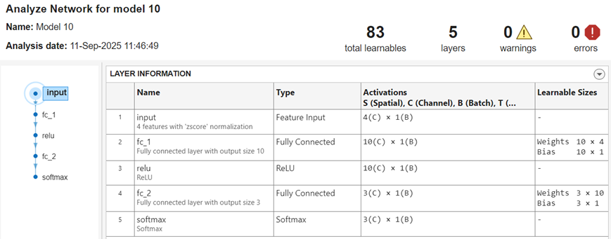
After you train a neural network classifier, you can display its network architecture and layer information. In the Plots and Results section of the Learn tab, click the arrow to open the gallery, and then click Analyze Network in the Neural Network Results group. This option is also available in the Network Architecture section of the Summary tab.
The app displays information about each layer in the network. For more
information about neural network layers, see the fitcnet function page and the topic List of Deep Learning Layers (Deep Learning Toolbox).
Neural Network Model Hyperparameter Options
Neural network classifiers in Classification Learner use the fitcnet function. You can set these options:
Number of fully connected layers — Specify the number of fully connected layers in the neural network, excluding the final fully connected layer for classification. You can choose a maximum of three fully connected layers. If you require a network with more layers and have a Deep Learning Toolbox license, you can use a customizable preset instead. See Customizable Neural Network Classifiers.
First layer size, Second layer size, and Third layer size — Specify the size of each fully connected layer, excluding the final fully connected layer. If you choose to create a neural network with multiple fully connected layers, consider specifying layers with decreasing sizes.
Activation — Specify the activation function for all fully connected layers, excluding the final fully connected layer. The activation function for the last fully connected layer is always softmax. Choose from the following activation functions:
ReLU,Tanh,None, andSigmoid.Iteration limit — Specify the maximum number of training iterations.
Regularization strength (Lambda) — Specify the ridge (L2) regularization penalty term.
Standardize data — Specify whether to standardize the numeric predictors. If predictors have widely different scales, standardizing can improve the fit. Standardizing the data is highly recommended.
Alternatively, you can let the app choose some of these model options automatically by using hyperparameter optimization. See Hyperparameter Optimization in Classification Learner App.
View Training Progress Plots for Neural Network
After you train a regular or customizable neural network classifier, you can view plots that show how the training progressed. In the Plots and Results section, click the arrow to open the gallery, and then click Training Progress in the Neural Network Results group.
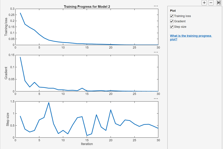
In the Plot pane, you can select check boxes to display
the cross-entropy training loss, optimization gradient, and step size values at
each training iteration. You can use these plots to assess model optimization
convergence and to check for possible overfitting. For more information about
neural network training parameters, see the fitcnet function page.
Customizable Neural Network Classifiers
Since R2026a
If you have a Deep Learning Toolbox license, you can select two additional presets for neural network classifiers:
Fully connected customizable neural network — A customizable fully connected network that is similar to the Bilayered and Trilayered Neural Network presets, but has five fully connected layers.
Residual customizable neural network — A customizable network that contains one residual connection. Residual connections improve gradient flow through the network and enable you to train deeper networks.
Note
When working with customizable neural network classifiers, you cannot perform hyperparameter optimization or export a trained model to MATLAB Coder™ or Simulink®.
Display and Customize Network Architecture
After you create a customizable neural network classifier, the Summary tab displays the network architecture.
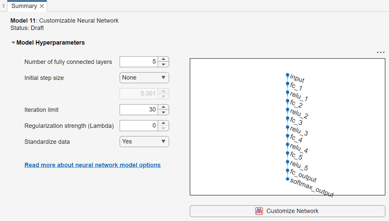
You can customize the network architecture by adding or removing layers, and editing layer properties. Click the Customize Network button to launch the Network Editor, a basic version of the Deep Network Designer (Deep Learning Toolbox) app that contains a subset of the layers listed in List of Deep Learning Layers (Deep Learning Toolbox). In the Network Editor, you cannot analyze a network for compression, or import a network from a file or the MATLAB workspace.
For a detailed example showing how to customize a neural network using the Network Editor, see Edit Customizable Neural Network Using Network Editor in Classification Learner or Regression Learner.
Analyze Network
You can display information about the layers in a customizable neural network by clicking Analyze Network in the Plots and Results section of the Learn tab. After you train the model, this option is also available in the Network Architecture section of the Summary tab.
To analyze your network while in the Network Editor, click Analyze in the Analysis section of the Designer tab. The app displays information about the layers, and checks the network for errors that prevent the model from being trained. Some common errors include size mismatches, missing connections, and missing layers. If your network contains errors, you can fix them using options in the Designer tab.
Set Hyperparameter Options
In the Model Hyperparameters section of the Summary tab, you can set these hyperparameters:
Number of fully connected layers — Specify the number of fully connected layers in the neural network, excluding the final fully connected layer for classification. This option is not available after you make any changes to the network in Network Editor. This option is also not available for the Residual Customizable Neural Network classifier preset.
Initial step size — Select one of these options:
Manual — Specify an initial step size to determine the initial Hessian approximation used in training the model. The default value is
0.001.Auto — The app determines the initial step size automatically.
None (default) — Do not use an initial step size.
Iteration limit — Specify the maximum number of training iterations.
Regularization strength (Lambda) — Specify the ridge (L2) regularization penalty term.
Standardize data — Specify whether to standardize the numeric predictors. If the predictors have widely different scales, standardizing can improve the fit. Standardizing the data is highly recommended. Note that because Classification Learner performs the data standardization, the Normalization value of a featureInputLayer block must be
"none"in a customizable neural network classifier.
For more information on these hyperparameters, see the fitcnet function page.
See Also
Topics
- Edit Customizable Neural Network Using Network Editor in Classification Learner or Regression Learner
- Train Classification Models in Classification Learner App
- Start a Classification Learner or Regression Learner Session
- Feature Selection and Feature Transformation Using Classification Learner App
- Visualize and Assess Classifier Performance in Classification Learner
- Export Classification Model to Predict New Data