loss

R2026b

Classification loss for linear classification models

Syntax

L = loss(Mdl,X,Y)

L = loss(Mdl,Tbl,ResponseVarName)

L = loss(Mdl,Tbl,Y)

L = loss(___,Name=Value)

Description

L = loss(Mdl,X,Y) returns the classification losses for the binary, linear classification model Mdl using predictor data in X and corresponding class labels in Y. L contains classification error rates for each regularization strength in Mdl.

L = loss(Mdl,Tbl,ResponseVarName) returns the classification losses for the predictor data in Tbl and the true class labels in Tbl.ResponseVarName.

L = loss(Mdl,Tbl,Y) returns the classification losses for the predictor data in table Tbl and the true class labels in Y.

L = loss(___,Name=Value) specifies options using one or more name-value arguments in addition to any of the input argument combinations in previous syntaxes. For example, you can specify that columns in the predictor data correspond to observations or specify the classification loss function.

Examples

Estimate Test-Sample Classification Loss

Load the NLP data set.

load nlpdata

X is a sparse matrix of predictor data, and Y is a categorical vector of class labels. There are more than two classes in the data.

The models should identify whether the word counts in a web page are from the Statistics and Machine Learning Toolbox™ documentation. So, identify the labels that correspond to the Statistics and Machine Learning Toolbox™ documentation web pages.

Ystats = Y == "stats";

Train a binary, linear classification model that can identify whether the word counts in a documentation web page are from the Statistics and Machine Learning Toolbox™ documentation. Specify to hold out 30% of the observations. Optimize the objective function using SpaRSA.

rng(1) % For reproducibility 
CVMdl = fitclinear(X,Ystats,Solver="sparsa",Holdout=0.30);
CMdl = CVMdl.Trained{1};

CVMdl is a ClassificationPartitionedLinear model. It contains the property Trained, which is a 1-by-1 cell array holding a ClassificationLinear model that the software trained using the training set.

Extract the training and test data from the partition definition.

trainIdx = training(CVMdl.Partition);
testIdx = test(CVMdl.Partition);

Estimate the training- and test-sample classification error.

ceTrain = loss(CMdl,X(trainIdx,:),Ystats(trainIdx))

ceTrain = 
1.3572e-04

ceTest = loss(CMdl,X(testIdx,:),Ystats(testIdx))

ceTest = 
5.2804e-04

Because there is one regularization strength in CMdl, ceTrain and ceTest are numeric scalars.

Specify Custom Classification Loss

Load the NLP data set. Preprocess the data as in Estimate Test-Sample Classification Loss, and transpose the predictor data.

load nlpdata
Ystats = Y == "stats";
X = X';

Train a binary, linear classification model. Specify to hold out 30% of the observations. Optimize the objective function using SpaRSA. Specify that the predictor observations correspond to columns.

rng(1) % For reproducibility 
CVMdl = fitclinear(X,Ystats,Solver="sparsa",Holdout=0.30, ...
    ObservationsIn="columns");
CMdl = CVMdl.Trained{1};

CVMdl is a ClassificationPartitionedLinear model. It contains the property Trained, which is a 1-by-1 cell array holding a ClassificationLinear model that the software trained using the training set.

Extract the training and test data from the partition definition.

trainIdx = training(CVMdl.Partition);
testIdx = test(CVMdl.Partition);

Create an anonymous function that measures linear loss, that is,

$$L=\frac{\sum _j-w_j{y}_j{f}_j}{\sum _j{w}_j}.$$

$$w_j$$ is the weight for observation j, $$y_j$$ is response j (-1 for the negative class, and 1 otherwise), and $$f_j$$ is the raw classification score of observation j. Custom loss functions must be written in a particular form. For rules on writing a custom loss function, see the LossFun name-value argument.

linearloss = @(C,S,W,Cost)sum(-W.*sum(S.*C,2))/sum(W);

Estimate the training- and test-sample classification loss using the linear loss function.

ceTrain = loss(CMdl,X(:,trainIdx),Ystats(trainIdx),LossFun=linearloss, ...
    ObservationsIn="columns")

ceTrain = 
-7.8330

ceTest = loss(CMdl,X(:,testIdx),Ystats(testIdx),LossFun=linearloss, ...
    ObservationsIn="columns")

ceTest = 
-7.7383

Find Good Lasso Penalty Using Classification Loss

To determine a good lasso-penalty strength for a linear classification model that uses a logistic regression learner, compare test-sample classification error rates.

Load the NLP data set. Preprocess the data as in Specify Custom Classification Loss.

load nlpdata
Ystats = Y == "stats";
X = X'; 

rng(10) % For reproducibility
Partition = cvpartition(Ystats,Holdout=0.30);
testIdx = test(Partition);
XTest = X(:,testIdx);
YTest = Ystats(testIdx);

Create a set of 11 logarithmically-spaced regularization strengths from $$10^{-6}$$ through $$10^{-0.5}$$.

Lambda = logspace(-6,-0.5,11);

Train binary, linear classification models that use each of the regularization strengths. Optimize the objective function using SpaRSA. Lower the tolerance on the gradient of the objective function to 1e-8.

CVMdl = fitclinear(X,Ystats,ObservationsIn="columns", ...
    CVPartition=Partition,Learner="logistic",Solver="sparsa", ...
    Regularization="lasso",Lambda=Lambda,GradientTolerance=1e-8)

CVMdl = 
  ClassificationPartitionedLinear
    CrossValidatedModel: 'Linear'
           ResponseName: 'Y'
        NumObservations: 31572
                  KFold: 1
              Partition: [1×1 cvpartition]
             ClassNames: [0 1]
         ScoreTransform: 'none'


  Properties, Methods

Extract the trained linear classification model.

Mdl = CVMdl.Trained{1}

Mdl = 
  ClassificationLinear
      ResponseName: 'Y'
        ClassNames: [0 1]
    ScoreTransform: 'logit'
              Beta: [34023×11 double]
              Bias: [-12.1623 -12.1623 -12.1623 -12.1623 -12.1623 -6.2503 -5.0651 -4.2165 -3.3990 -3.2452 -2.9783]
            Lambda: [1.0000e-06 3.5481e-06 1.2589e-05 4.4668e-05 1.5849e-04 5.6234e-04 0.0020 0.0071 0.0251 0.0891 0.3162]
           Learner: 'logistic'


  Properties, Methods

Mdl is a ClassificationLinear model object. Because Lambda is a sequence of regularization strengths, you can think of Mdl as 11 models, one for each regularization strength in Lambda.

Estimate the test-sample classification error.

ce = loss(Mdl,X(:,testIdx),Ystats(testIdx),ObservationsIn="columns");

Because there are 11 regularization strengths, ce is a 1-by-11 vector of classification error rates.

Higher values of Lambda lead to predictor variable sparsity, which is a good quality of a classifier. For each regularization strength, train a linear classification model using the entire data set and the same options as when you cross-validated the models. Determine the number of nonzero coefficients per model.

Mdl = fitclinear(X,Ystats,ObservationsIn="columns", ...
    Learner="logistic",Solver="sparsa",Regularization="lasso", ...
    Lambda=Lambda,GradientTolerance=1e-8);
numNZCoeff = sum(Mdl.Beta~=0);

In the same figure, plot the test-sample error rates and frequency of nonzero coefficients for each regularization strength. Plot all variables on the log scale.

figure
yyaxis left
plot(log10(Lambda),log10(ce),"-o")
ylabel("log_{10} classification error")

yyaxis right
plot(log10(Lambda),log10(numNZCoeff + 1),"-o")
ylabel("log_{10} nonzero-coefficient frequency")

xlabel("log_{10} Lambda")
title("Test-Sample Statistics")

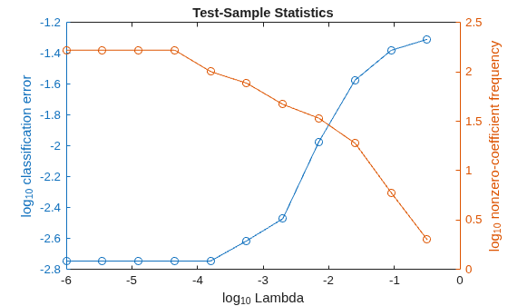
Choose the index of the regularization strength that balances predictor variable sparsity and low classification error. In this case, a value between $$10^{-4}$$ to $$10^{-1}$$ should suffice.

idxFinal = 7;

Select the model from Mdl with the chosen regularization strength.

MdlFinal = selectModels(Mdl,idxFinal);

MdlFinal is a ClassificationLinear model containing one regularization strength. To estimate labels for new observations, pass MdlFinal and the new data to predict.

Input Arguments

Mdl — Binary, linear classification model

ClassificationLinear model object

Binary, linear classification model, specified as a ClassificationLinear model object. You can create a ClassificationLinear model object using fitclinear.

X — Predictor data

full matrix | sparse matrix

Predictor data, specified as an n-by-p full or sparse matrix. This orientation of X indicates that rows correspond to individual observations, and columns correspond to individual predictor variables.

Note

If you orient your predictor matrix so that observations correspond to columns and specify ObservationsIn="columns", then you might experience a significant reduction in computation time.

The length of Y and the number of observations in X must be equal.

Data Types: single | double

Y — Class labels

categorical array | character array | string array | logical vector | numeric vector | cell array of character vectors

Class labels, specified as a categorical, character, or string array; logical or numeric vector; or cell array of character vectors.

• The data type of Y must be the same as the data type of Mdl.ClassNames. (The software treats string arrays as cell arrays of character vectors.)

• The distinct classes in Y must be a subset of Mdl.ClassNames.

• If Y is a character array, then each element must correspond to one row of the array.

• The length of Y must be equal to the number of observations in X or Tbl.

Data Types: categorical | char | string | logical | single | double | cell

Tbl — Sample data

table

Sample data used to train the model, specified as a table. Each row of Tbl corresponds to one observation, and each column corresponds to one predictor variable. Optionally, Tbl can contain additional columns for the response variable and observation weights. Tbl must contain all the predictors used to train Mdl. Multicolumn variables and cell arrays other than cell arrays of character vectors are not allowed.

If Tbl contains the response variable used to train Mdl, then you do not need to specify ResponseVarName or Y.

If you train Mdl using sample data contained in a table, then the input data for loss must also be in a table.

ResponseVarName — Response variable name

name of variable in Tbl

Response variable name, specified as the name of a variable in Tbl. If Tbl contains the response variable used to train Mdl, then you do not need to specify ResponseVarName.

If you specify ResponseVarName, then you must specify it as a character vector or string scalar. For example, if the response variable is stored as Tbl.Y, then specify ResponseVarName as "Y". Otherwise, the software treats all columns of Tbl, including Tbl.Y, as predictors.

The response variable must be a categorical, character, or string array; a logical or numeric vector; or a cell array of character vectors. If the response variable is a character array, then each element must correspond to one row of the array.

Data Types: char | string

Name-Value Arguments

Specify optional pairs of arguments as Name1=Value1,...,NameN=ValueN, where Name is the argument name and Value is the corresponding value. Name-value arguments must appear after other arguments, but the order of the pairs does not matter.

Example: loss(Mdl,Tbl,"Response",LossFun="hinge") specifies to compute the hinge loss for the model Mdl.

LossFun — Loss function

"classiferror" (default) | "binodeviance" | "classifcost" | "exponential" | "hinge" | "logit" | "mincost" | "quadratic" | function handle

Loss function, specified as a built-in loss function name or function handle.

• The following table lists the available loss functions. Specify one using its corresponding character vector or string scalar.

  Value	Description
  "binodeviance"	Binomial deviance
  "classifcost"	Observed misclassification cost
  "classiferror"	Misclassified rate in decimal
  "exponential"	Exponential loss
  "hinge"	Hinge loss
  "logit"	Logistic loss
  "mincost"	Minimal expected misclassification cost (for classification scores that are posterior probabilities)
  "quadratic"	Quadratic loss

  "mincost" is appropriate for classification scores that are posterior probabilities. For linear classification models, logistic regression learners return posterior probabilities as classification scores by default, but SVM learners do not (see predict).

• To specify a custom loss function, use function handle notation. The function must have this form:

  lossvalue = lossfun(C,S,W,Cost)

  • The output argument lossvalue is a scalar.

  • You specify the function name (lossfun).

  • C is an n-by-K logical matrix with rows indicating the class to which the corresponding observation belongs. n is the number of observations in Tbl or X, and K is the number of distinct classes (numel(Mdl.ClassNames)). The column order corresponds to the class order in Mdl.ClassNames. Create C by setting C(p,q) = 1, if observation p is in class q, for each row. Set all other elements of row p to 0.

  • S is an n-by-K numeric matrix of classification scores. The column order corresponds to the class order in Mdl.ClassNames. S is a matrix of classification scores, similar to the output of predict.

  • W is an n-by-1 numeric vector of observation weights.

  • Cost is a K-by-K numeric matrix of misclassification costs. For example, Cost = ones(K) – eye(K) specifies a cost of 0 for correct classification and 1 for misclassification.

Example: LossFun=@lossfun

Data Types: char | string | function_handle

ObservationsIn — Predictor data observation dimension

"rows" (default) | "columns"

Predictor data observation dimension, specified as "rows" or "columns".

Note

If you orient your predictor matrix so that observations correspond to columns and specify ObservationsIn="columns", then you might experience a significant reduction in computation time. You cannot specify ObservationsIn="columns" for predictor data in a table.

Example: ObservationsIn="columns"

Data Types: char | string

Prior — Class weights

Mdl.Prior (default) | "empirical" | "uniform" | numeric vector

Since R2026b

Class weights, or prior probabilities, specified as "empirical", "uniform", or a numeric vector.

Value	Description
"empirical"	loss uses the class frequencies in Y or Tbl.ResponseVarName. The function returns an unweighted loss, with respect to class.
"uniform"	loss assigns a weight of 1/K to each class, where K is the number of classes.
Numeric vector	Specify a custom weight for each class. The sum of the weights must equal 1.

By default, loss uses the class prior probabilities specified in the Prior property of the classification model.

Example: Prior="empirical"

Data Types: single | double | char | string

Weights — Observation weights

ones(size(X,1),1) (default) | numeric vector | name of variable in Tbl

Observation weights, specified as a numeric vector or the name of a variable in Tbl.

• If you specify Weights as a numeric vector, then the size of Weights must be equal to the number of observations in X or Tbl.

• If you specify Weights as the name of a variable in Tbl, then the name must be a character vector or string scalar. For example, if the weights are stored as Tbl.W, then specify Weights as "W". Otherwise, the software treats all columns of Tbl, including Tbl.W, as predictors.

If you supply weights, then for each regularization strength, loss computes the weighted classification loss and normalizes weights to sum up to the value of the prior probability in the respective class.

Data Types: double | single

Output Arguments

L — Classification losses

numeric scalar | numeric row vector

Classification losses, returned as a numeric scalar or row vector. The interpretation of L depends on LossFun, Prior, and Weights.

L is the same size as Mdl.Lambda. L(j) is the classification loss of the linear classification model trained using the regularization strength Mdl.Lambda(j).

For more information, see Classification Loss.

More About

Classification Loss

Classification loss functions measure the predictive inaccuracy of classification models. When you compare the same type of loss among many models, a lower loss indicates a better predictive model.

Consider the following scenario.

• L is the weighted average classification loss.

• n is the sample size.

• y_j is the observed class label. The software codes it as –1 or 1, indicating the negative or positive class (or the first or second class in the ClassNames property), respectively.

• f(X_j) is the positive-class classification score for observation (row) j of the predictor data X.

• m_j = y_jf(X_j) is the classification score for classifying observation j into the class corresponding to y_j. Positive values of m_j indicate correct classification and do not contribute much to the average loss. Negative values of m_j indicate incorrect classification and contribute significantly to the average loss.

• The weight for observation j is w_j . The software normalizes the observation weights so that they sum to the corresponding class weights (prior probabilities) specified by the Prior name-value argument. Therefore,

  $${\displaystyle \sum _{j=1}^n{w}_j}=1.$$

Given this scenario, the following table describes the supported loss functions that you can specify by using the LossFun name-value argument.

Loss Function	Value of LossFun	Equation
Binomial deviance	"binodeviance"	$$L={\displaystyle \sum _{j=1}^n{w}_j\log \left\{1+\exp \left[-2m_j\right]\right\}}.$$
Observed misclassification cost	"classifcost"	$$L={\displaystyle \sum _{j=1}^n{w}_j}{c}_{y_j{\widehat{y}}_j},$$ where $${\widehat{y}}_j$$ is the class label corresponding to the class with the maximal score, and $$c_{y_j{\widehat{y}}_j}$$ is the user-specified cost of classifying an observation into class $${\widehat{y}}_j$$ when its true class is yj.
Misclassified rate in decimal	"classiferror"	$$L={\displaystyle \sum _{j=1}^n{w}_j}I\left\{{\widehat{y}}_j\ne y_j\right\},$$ where I{·} is the indicator function.
Cross-entropy loss	"crossentropy"	"crossentropy" is appropriate only for neural network models. The weighted cross-entropy loss is $$L=-{\displaystyle \sum _{j=1}^n\frac{{\tilde{w}}_j\log (m_j)}{Kn}},$$ where the weights $${\tilde{w}}_j$$ are normalized to sum to n instead of 1.
Exponential loss	"exponential"	$$L={\displaystyle \sum _{j=1}^n{w}_j\exp \left(-m_j\right)}.$$
Hinge loss	"hinge"	$$L={\displaystyle \sum }_{j=1}^n{w}_j\max \left\{0,1-m_j\right\}.$$
Logistic loss	"logit"	$$L={\displaystyle \sum _{j=1}^n{w}_j\log \left(1+\exp \left(-m_j\right)\right)}.$$
Minimal expected misclassification cost	"mincost"	"mincost" is appropriate only if classification scores are posterior probabilities. The software computes the weighted minimal expected classification cost using this procedure for observations j = 1,...,n. Estimate the expected misclassification cost of classifying the observation Xj into the class k: $${\gamma }_{jk}={\left(f{\left(X_j\right)}^{\prime }C\right)}_k.$$ f(Xj) is the column vector of class posterior probabilities for the observation Xj. C is the cost matrix stored in the Cost property of the model. For observation j, predict the class label corresponding to the minimal expected misclassification cost: $${\widehat{y}}_j=\underset{k=1,\mathrm{...},K}{\text{argmin}}{\gamma }_{jk}.$$ Using C, identify the cost incurred (cj) for making the prediction. The weighted average of the minimal expected misclassification cost loss is $$L={\displaystyle \sum _{j=1}^n{w}_j{c}_j}.$$
Quadratic loss	"quadratic"	$$L={\displaystyle \sum _{j=1}^n{w}_j{\left(1-m_j\right)}^2}.$$

If you use the default cost matrix (whose element value is 0 for correct classification and 1 for incorrect classification), then the loss values for "classifcost", "classiferror", and "mincost" are identical. For a model with a nondefault cost matrix, the "classifcost" loss is equivalent to the "mincost" loss most of the time. These losses can be different if prediction into the class with maximal posterior probability is different from prediction into the class with minimal expected cost. Note that "mincost" is appropriate only if classification scores are posterior probabilities.

This figure compares the loss functions (except "classifcost", "crossentropy", and "mincost") over the score m for one observation. Some functions are normalized to pass through the point (0,1).

Tips

• By default, loss uses the class probabilities specified during training (which are stored in the Prior property of the classification model) to compute the classification loss. To return the class-unweighted loss, specify Prior="empirical". (since R2026b)

• If the predictor data in X or Tbl contains any missing values and LossFun is not set to "classifcost", "classiferror", or "mincost", the loss function might return NaN. (since R2022a)

  If loss in your code returns NaN, you can update your code to avoid this result by doing one of the following:

  • Remove or replace the missing values by using rmmissing or fillmissing, respectively.

  • Specify the name-value argument LossFun as "classifcost", "classiferror", or "mincost".

Extended Capabilities

Tall Arrays

Calculate with arrays that have more rows than fit in memory.

The loss function supports tall arrays with the following usage notes and limitations:

• loss does not support tall table data.

For more information, see Tall Arrays.

GPU Arrays

Accelerate code by running on a graphics processing unit (GPU) using Parallel Computing Toolbox™.

This function fully supports GPU arrays. For more information, see Run MATLAB Functions on a GPU (Parallel Computing Toolbox).

Version History

Introduced in R2016a

R2026b: Compute the class-unweighted loss

Compute the class-unweighted loss by setting the Prior name-value argument to "empirical" in the call to loss. You can also compute a class-weighted loss by setting Prior to the value "uniform" or a numeric vector whose entries sum to 1.

R2024a: Specify GPU arrays (requires Parallel Computing Toolbox)

loss fully supports GPU arrays.

R2022a: loss returns a different value for a model with a nondefault cost matrix

If you specify a nondefault cost matrix when you train the input model object, the loss function returns a different value compared to previous releases.

The loss function uses the prior probabilities stored in the Prior property to normalize the observation weights of the input data. Also, the function uses the cost matrix stored in the Cost property if you specify the LossFun name-value argument as "classifcost" or "mincost". The way the function uses the Prior and Cost property values has not changed. However, the property values stored in the input model object have changed for a model with a nondefault cost matrix, so the function might return a different value.

For details about the property value change, see Cost property stores the user-specified cost matrix.

If you want the software to handle the cost matrix, prior probabilities, and observation weights in the same way as in previous releases, adjust the prior probabilities and observation weights for the nondefault cost matrix, as described in Adjust Prior Probabilities and Observation Weights for Misclassification Cost Matrix. Then, when you train a classification model, specify the adjusted prior probabilities and observation weights by using the Prior and Weights name-value arguments, respectively, and use the default cost matrix.

R2022a: loss can return NaN for predictor data with missing values

The loss function no longer omits an observation with a NaN score when computing the weighted average classification loss. Therefore, loss can now return NaN when the predictor data X or the predictor variables in Tbl contain any missing values, and the name-value argument LossFun is not specified as "classifcost", "classiferror", or "mincost". In most cases, if the test set observations do not contain missing predictors, the loss function does not return NaN.

This change improves the automatic selection of a classification model when you use fitcauto. Before this change, the software might select a model (expected to best classify new data) with few non-NaN predictors.

If loss in your code returns NaN, you can update your code to avoid this result by doing one of the following:

• Remove or replace the missing values by using rmmissing or fillmissing, respectively.

• Specify the name-value argument LossFun as "classifcost", "classiferror", or "mincost".

The following table shows the classification models for which the loss object function might return NaN. For more details, see the Compatibility Considerations for each loss function.

Model Type	Full or Compact Model Object	loss Object Function
Discriminant analysis classification model	ClassificationDiscriminant, CompactClassificationDiscriminant	loss
Ensemble of learners for classification	ClassificationEnsemble, CompactClassificationEnsemble	loss
Gaussian kernel classification model	ClassificationKernel	loss
k-nearest neighbor classification model	ClassificationKNN	loss
Linear classification model	ClassificationLinear	loss
Neural network classification model	ClassificationNeuralNetwork, CompactClassificationNeuralNetwork	loss
Support vector machine (SVM) classification model	ClassificationSVM, CompactClassificationSVM	loss