Main Content

relieff

Rank importance of predictors using ReliefF or RReliefF algorithm

Description

example

[idx,weights] = relieff(X,y,k) ranks predictors using either the ReliefF or RReliefF algorithm with k nearest neighbors. The input matrix X contains predictor variables, and the vector y contains a response vector. The function returns idx, which contains the indices of the most important predictors, and weights, which contains the weights of the predictors.

If y is numeric, relieff performs RReliefF analysis for regression by default. Otherwise, relieff performs ReliefF analysis for classification using k nearest neighbors per class. For more information on ReliefF and RReliefF, see Algorithms.

example

[idx,weights] = relieff(X,y,k,Name,Value) specifies additional options using one or more name-value pair arguments. For example, 'updates',10 sets the number of observations randomly selected for computing weights to 10.

Examples

collapse all

Load the sample data.

load fisheriris

Find the important predictors using 10 nearest neighbors.

[idx,weights] = relieff(meas,species,10)
idx = 1×4

     4     3     1     2

weights = 1×4

    0.1399    0.1226    0.3590    0.3754

idx shows the predictor numbers listed according to their ranking. The fourth predictor is the most important, and the second predictor is the least important. weights gives the weight values in the same order as the predictors. The first predictor has a weight of 0.1399, and the fourth predictor has a weight of 0.3754.

Load the sample data.

load ionosphere

Rank the predictors based on importance using 10 nearest neighbors.

[idx,weights] = relieff(X,Y,10);

Create a bar plot of predictor importance weights.

bar(weights(idx))
xlabel('Predictor rank')
ylabel('Predictor importance weight')

Figure contains an axes object. The axes object with xlabel Predictor rank, ylabel Predictor importance weight contains an object of type bar.

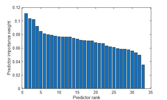
Select the top 5 most important predictors. Find the columns of these predictors in X.

idx(1:5)
ans = 1×5

    24     3     8     5    14

The 24th column of X is the most important predictor of Y.

Rank categorical predictors using relieff.

Load the sample data.

load carbig

Convert the categorical predictor variables Mfg, Model, and Origin to numerical values, and combine them into an input matrix. Specify the response variable MPG.

X = [grp2idx(Mfg) grp2idx(Model) grp2idx(Origin)];
y = MPG;

Find the ranks and weights of the predictor variables using 10 nearest neighbors and treating the data in X as categorical.

[idx,weights] = relieff(X,y,10,'categoricalx','on')
idx = 1×3

     2     3     1

weights = 1×3

   -0.0019    0.0501    0.0114

The Model predictor is the most important in predicting MPG. The Mfg variable has a negative weight, indicating it is not a good predictor of MPG.

Input Arguments

collapse all

Predictor data, specified as a numeric matrix. Each row of X corresponds to one observation, and each column corresponds to one variable.

Data Types: single | double

Response data, specified as a numeric vector, categorical vector, logical vector, character array, string array, or cell array of character vectors.

Data Types: single | double | categorical | logical | char | string | cell

Number of nearest neighbors, specified as a positive integer scalar.

Data Types: single | double

Name-Value Arguments

Specify optional pairs of arguments as Name1=Value1,...,NameN=ValueN, where Name is the argument name and Value is the corresponding value. Name-value arguments must appear after other arguments, but the order of the pairs does not matter.

Before R2021a, use commas to separate each name and value, and enclose Name in quotes.

Example: relieff(X,y,5,'method','classification','categoricalx','on') specifies 5 nearest neighbors and treats the response variable and predictor data as categorical.

Method for computing weights, specified as the comma-separated pair consisting of 'method' and either 'regression' or 'classification'. If y is numeric, 'regression' is the default method. Otherwise, 'classification' is the default.

Example: 'method','classification'

Prior probabilities for each class, specified as the comma-separated pair consisting of 'prior' and a value in this table.

ValueDescription
'empirical'The class probabilities are determined from class frequencies in y.
'uniform'All class probabilities are equal.
numeric vectorOne value exists for each distinct group name.
structure

A structure S with two fields:

  • S.group contains the group names as a variable of the same type as y.

  • S.prob contains a vector of corresponding probabilities.

Example: 'prior','uniform'

Data Types: single | double | char | string | struct

Number of observations to select at random for computing weights, specified as the comma-separated pair consisting of 'updates' and either 'all' or a positive integer scalar. By default, relieff uses all observations.

Example: 'updates',25

Data Types: single | double | char | string

Categorical predictors flag, specified as the comma-separated pair consisting of 'categoricalx' and either 'on' or 'off'. If you specify 'on', then relieff treats all predictors in X as categorical. Otherwise, it treats all predictors in X as numeric. You cannot mix numeric and categorical predictors.

Example: 'categoricalx','on'

Distance scaling factor, specified as the comma-separated pair consisting of 'sigma' and a numeric positive scalar. For observation i, influence on the predictor weight from its nearest neighbor j is multiplied by e(rank(i,j)/sigma)2. rank(i,j) is the position of the jth observation among the nearest neighbors of the ith observation, sorted by distance. The default is Inf for classification (all nearest neighbors have the same influence) and 50 for regression.

Example: 'sigma',20

Data Types: single | double

Output Arguments

collapse all

Indices of predictors in X ordered by predictor importance, returned as a numeric vector. For example, if idx(3) is 5, then the third most important predictor is the fifth column in X.

Data Types: double

Weights of the predictors, returned as a numeric vector. The values in weights have the same order as the predictors in X. weights range from –1 to 1, with large positive weights assigned to important predictors.

Data Types: double

Tips

  • Predictor ranks and weights usually depend on k. If you set k to 1, then the estimates can be unreliable for noisy data. If you set k to a value comparable with the number of observations (rows) in X, relieff can fail to find important predictors. You can start with k = 10 and investigate the stability and reliability of relieff ranks and weights for various values of k.

  • relieff removes observations with NaN values.

Algorithms

collapse all

ReliefF

ReliefF finds the weights of predictors in the case where y is a multiclass categorical variable. The algorithm penalizes the predictors that give different values to neighbors of the same class, and rewards predictors that give different values to neighbors of different classes.

ReliefF first sets all predictor weights Wj to 0. Then, the algorithm iteratively selects a random observation xr, finds the k-nearest observations to xr for each class, and updates, for each nearest neighbor xq, all the weights for the predictors Fj as follows:

If xr and xq are in the same class,

Wji=Wji1Δj(xr,xq)mdrq.

If xr and xq are in different classes,

Wji=Wji1+pyq1pyrΔj(xr,xq)mdrq.

  • Wji is the weight of the predictor Fj at the ith iteration step.

  • pyr is the prior probability of the class to which xr belongs, and pyq is the prior probability of the class to which xq belongs.

  • m is the number of iterations specified by 'updates'.

  • Δj(xr,xq) is the difference in the value of the predictor Fj between observations xr and xq. Let xrj denote the value of the jth predictor for observation xr, and let xqj denote the value of the jth predictor for observation xq.

    • For discrete Fj,

      Δj(xr,xq)={0,xrj=xqj1,xrjxqj.

    • For continuous Fj,

      Δj(xr,xq)=|xrjxqj|max(Fj)min(Fj).

  • drq is a distance function of the form

    drq=d˜rql=1kd˜rl.

    The distance is subject to the scaling

    d˜rq=e(rank(r,q)/sigma)2

    where rank(r,q) is the position of the qth observation among the nearest neighbors of the rth observation, sorted by distance. k is the number of nearest neighbors, specified by k. You can change the scaling by specifying 'sigma'.

RReliefF

RReliefF works with continuous y. Similar to ReliefF, RReliefF also penalizes the predictors that give different values to neighbors with the same response values, and rewards predictors that give different values to neighbors with different response values. However, RReliefF uses intermediate weights to compute the final predictor weights.

Given two nearest neighbors, assume the following:

  • Wdy is the weight of having different values for the response y.

  • Wdj is the weight of having different values for the predictor Fj.

  • Wdydj is the weight of having different response values and different values for the predictor Fj.

RReliefF first sets the weights Wdy, Wdj, Wdydj, and Wj equal to 0. Then, the algorithm iteratively selects a random observation xr, finds the k-nearest observations to xr, and updates, for each nearest neighbor xq, all the intermediate weights as follows:

Wdyi=Wdyi1+Δy(xr,xq)drq.

Wdji=Wdji1+Δj(xr,xq)drq.

Wdydji=Wdydji1+Δy(xr,xq)Δj(xr,xq)drq.

  • The i and i-1 superscripts denote the iteration step number. m is the number of iterations specified by 'updates'.

  • Δy(xr,xq) is the difference in the value of the continuous response y between observations xr and xq. Let yr denote the value of the response for observation xr, and let yq denote the value of the response for observation xq.

    Δy(xr,xq)=|yryq|max(y)min(y).

  • The Δj(xr,xq) and drq functions are the same as for ReliefF.

RReliefF calculates the predictor weights Wj after fully updating all the intermediate weights.

Wj=WdydjWdyWdjWdydjmWdy.

For more information, see [2].

References

[1] Kononenko, I., E. Simec, and M. Robnik-Sikonja. (1997). “Overcoming the myopia of inductive learning algorithms with RELIEFF.” Retrieved from CiteSeerX: https://link.springer.com/article/10.1023/A:1008280620621

[2] Robnik-Sikonja, M., and I. Kononenko. (1997). “An adaptation of Relief for attribute estimation in regression.” Retrieved from CiteSeerX: https://www.semanticscholar.org/paper/An-adaptation-of-Relief-for-attribute-estimation-in-Robnik-Sikonja-Kononenko/9548674b6a3c601c13baa9a383d470067d40b896

[3] Robnik-Sikonja, M., and I. Kononenko. (2003). “Theoretical and empirical analysis of ReliefF and RReliefF.” Machine Learning, 53, 23–69.

Version History

Introduced in R2010b