Results for
The toughest problem in the Cody Contest 2025 is Clueless - Lord Ned in the Game Room. Thank you Matt Tearle for such as wonderful problem. We can approach this clueless(!) tough problem systematically.
Initialize knowledge Matrix
Based on the hints provided in the problem description, we can initialize a knowledge matrix of size n*3 by m+1. The rows of the knowledge matrix represent the different cards and the columns represent the players. In the knowledge matrix, the first n rows represent category 1 cards, the next n rows, category 2 and the next category 3. We can initialize this matrix with zeros. On the go, once we know that a player holds the card, we can make that entry as 1 and if a player doesn't have the card, we can make that entry as -1.
yourcards processing
These are cards received by us.
- In the knowledge matrix, mark the entries as 1 for the cards received. These entries will be the some elements along the column pnum of the knowledge matrix.
- Mark all other entries along the column pnum as -1, as we don't receive other cards.
- Mark all other entries along the rows corresponding to the received cards as -1, as other players cannot receive the cards that are with us.
commoncards processing
These are the common cards kept open.
- In the knowledge matrix, mark the entries as 1 for the common cards. These entries will be some elements along the column (m+1) of the knowledge matrix.
- Mark all other entries along the column (m+1) as -1, as other cards are not common.
- Mark all other entries along the rows corresponding to the common cards as -1, as other players cannot receive the cards that are common.
Result -1 processing
In the turns input matrix, the result (5th column) value -1 means, the corresponding player doesn't have the 3 cards asked.
- Find all the rows with result as -1.
- For those corresponding players (1st element in each row of turns matrix), mark -1 entries in the knowledge matrix for those 3 absent cards.
pnum turns processing
These are our turns, so we get definite answers for the asked cards. Make sure to traverse only the rows corresponding to our turn.
- The results with -1 are already processed in the previous step.
- The results other than -1 means, that particular card is present with the asked player. So mark the entry as 1 for the corresponding player in the knowledge matrix.
- Mark all other entries along the row corresponding to step 2 as -1, as other players cannot receive this card.
Result 0 processing
So far, in the yourcards processing, commoncards processing, result -1 processing and pnum turns processing, we had very straightforward definite knowledge about the presence/absence of the card with a player. This step onwards, the tricky part of the problem begins.
result 0 means, any one (or more) of the asked cards are present with the asked player. We don't know exactly which card.
- For the asked player, if we have a definite no answer (-1 value in the knowledge matrix) for any two of the three asked cards, then we are sure about the card that is present with the player.
- Mark the entry as 1 for the definitely known card for the corresponding player in the knowledge matrix.
- Mark all other entries along the row corresponding to step 2 as -1, as other players cannot receive this card.
Cards per Player processing
Based on the number of cards present in the yourcards, we know the ncards, the number of cards per player.
Check along each column of the knowledge matrix, that is for each player.
- If the number of ones (definitely present cards) is equal to ncards, we can make all other entries along the column as -1, as this player cannot have any other card.
- If the sum of number of ones (definitely present cards) and the number of zeros (unknown cards) is equal to ncards, we can (i) mark the zero entries as one, as the unknown cards have become definitely present cards, (ii) mark all other entries along the column as -1, as other players cannot have any other card.
Category-wise cards checking
For each category, we must get a definite card to be present in the envelope.
- In each category (For every group of n rows of knowledge matrix), check for a row with all -1s. That is a card which is definitely not present with any of the players. Then this card will surely be present in the envelope. Add it to the output.
- If we could not find an all -1 row, then in that category, check each row for a 1 to be present. Note down the rows which doesn't have a 1. Those cards' players are still unknown. If we have only one such row (unknown card), then it must be in the envelope, as from each category one card is present in the envelope. Add it to the output.
- For the card identified in Step 2, mark all the entries along that row in the knowledge matrix as -1, as this card doesn't belong to any player.
Looping Over
In our so far steps, we could note that, the knowledge matrix got updated even after "Result 0 processing" step. This updation in the knowledge matrix may help the "Result 0 processing" step, if we perform it again. So, we can loop over the steps, "Result 0 processing", "Cards per Player processing" and "Category-wise cards checking" again. This ensures that, we will get the desired number of envelop cards (three in our case) as output.
The Cody Contest 2025 is underway, and it includes a super creative problem group which many of us have found fascinating. The central theme of the problems, expertly curated by @Matt Tearle, humorously revolves around the whims of the capricious dictator Lord Ned, as he goes out of his way to complicate the lives of his subjects and visitors alike. We cannot judge whether or not there's any truth to the rumors behind all the inside jokes, but it's obvious that the team had a lot of fun creating these; and we had even more fun solving them.
Today I want to showcase a way of graphically solving and visualizing one of those problems which I found very elegant, The Bridges of Nedsburg.
To briefly reiterate the problem, the number of islands and the arrangement of bridges of the city of Nedsburg are constantly changing. Lord Ned has decided to take advantage of this by charging visitors with an increasingly expensive n-bridge pass which allows them to cross up to n bridges in one journey. Given the Connectivity Matrix C, we are tasked with calculating the minimum n needed so that there is a path from every island to every other island in n steps or fewer.
Matt kindly provided us with some useful bit of math in the description detailing how to calculate the way to get from one island to another in an number of m steps. However, he has also hidden an alternative path to the solution in plain sight, in one of the graphs he provided. This involves the extremely useful and versatile class digraph, representing directed graphs, which have directional edges connecting the nodes. Here's some further great documentation and other cool resources on the topic for those who are interested in learning more about it:
Let's start using this class to explore a graphical solution to Lord Ned's conundrum. We will use the unit tests included in the problem to visualize the solution. We can retrieve the connectivity matrix for each case using the following function:
function C = getConnectivityMatrix(unit_test)
% Number of islands and bridge arrangement
switch unit_test
case 1
m = 3; idx = [3;4;8];
case 2
m = 3; idx = [3;4;7;8];
case 3
m = 4; idx = [2;7;8;10;13];
case 4
m = 4; idx = [4;5;7;8;9;14];
case 5
m = 5; idx = [5;8;11;12;14;18;22;23];
case 6
m = 5; idx = [2;5;8;14;20;21;24];
case 7
m = 6; idx = [3;4;7;11;18;23;24;26;30;32];
case 8
m = 6; idx = [3;11;12;13;18;19;28;32];
case 9
m = 7; idx = [3;4;6;8;13;14;20;21;23;31;36;47];
case 10
m = 7; idx = [4;11;13;14;19;22;23;26;28;30;34;35;37;38;45];
case 11
m = 8; idx = [2;4;5;6;8;12;13;17;27;39;44;48;54;58;60;62];
case 12
m = 8; idx = [3;9;12;20;24;29;30;31;33;44;48;50;53;54;58];
case 13
m = 9; idx = [8;9;10;14;15;22;25;26;29;33;36;42;44;47;48;50;53;54;55;67;80];
case 14
m = 9; idx = [8;10;22;32;37;40;43;45;47;53;56;57;62;64;69;70;73;77;79];
case 15
m = 10; idx = [2;5;8;13;16;20;24;27;28;36;43;49;53;62;71;75;77;83;86;87;95];
case 16
m = 10; idx = [4;9;14;21;22;35;37;38;44;47;50;51;53;55;59;61;63;66;69;76;77;84;85;86;90;97];
end
C = zeros(m);
C(idx) = 1;
end
The case in the example refers to unit test case 2.
unit_test = 2;
C = getConnectivityMatrix(unit_test);
disp(C)
D = digraph(C);
figure
p = plot(D,'LineWidth',1.5,'ArrowSize',10);
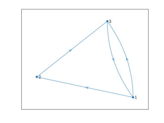
This is the same as the graph provided in the example. Another very useful method of digraph is shortestpath. This allows us to calculate the path and distance from one single node to another. For example:
% Path and distance from node 1 to node 2
[path12,dist12] = shortestpath(D,1,2);
fprintf('The shortest path from island %d to island %d is: %s. The minimum number of steps is: n = %d\n', 1, 2, join(string(path12), ' -> '),dist12)
% Path and distance from node 2 to node 1
[path21,dist21] = shortestpath(D,2,1);
fprintf('The shortest path from island %d to island %d is: %s. The minimum number of steps is: n = %d\n', 2, 1, join(string(path21), ' -> '),dist21)
figure
p = plot(D,'LineWidth',1.5,'ArrowSize',10);
highlight(p,path12,'EdgeColor','r','NodeColor','r','LineWidth',2)
highlight(p,path21,'EdgeColor',[0 0.8 0],'LineWidth',2)

But that's not all! digraph can also provide us with a matrix of the distances d, i.e. the steps needed to travel from island i to island j, where i and j are the rows and columns of d respectively. This is accomplished by using its distances method. The distance matrix can be visualized as:
d = distances(D);
figure
% Using pcolor w/ appending matrix workaround for convenience
pcolor([d,d(:,end);d(end,:),d(end,end)])
% Alternatively you can use imagesc(d), but you'll have to recreate the grid manually
axis square
set(gca,'YDir','reverse','XTick',[],'YTick',[])
[X,Y] = meshgrid(1:height(d));
text(X(:)+0.5,Y(:)+0.5,string(d(:)),'FontSize',11)
colormap(interp1(linspace(0,1,4), [1 1 1; 0.7 0.9 1; 0.6 0.7 1; 1 0.3 0.3], linspace(0,1,8)))
clim([-0.5 7+0.5])
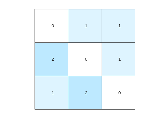
This confirms what we saw before, i.e. you need 1 step to go from island 1 to island 2, but 2 steps for vice versa. It also confirms that the minimum number of steps n that you need to buy the pass for is 2 (which also occurs for traveling from island 3 to island 2). As it's not the point of the post to give the full solution to the problem but rather present the graphical way of visualizing it I will not include the code of how to calculate this, but I'm sure that by now it's reduced to a trivial problem which you have already figured out how to solve.
That being said, now that we have the distance matrix, let's continue with the visualizations. First, let's plot the corresponding paths for each of these combinations:
figure
tiledlayout(size(C,1),size(C,2),'TileSpacing','tight','Padding','tight');
for i = 1:size(C,1)
for j = 1:size(C,2)
nexttile
p = plot(D,'ArrowSize',10);
highlight(p,shortestpath(D,i,j),'EdgeColor','r','NodeColor','r','LineWidth',2)
lims = axis;
text(lims(1)+diff(lims(1:2))*0.05,lims(3)+diff(lims(3:4))*0.9,sprintf('n = %d',d(i,j)))
end
end

This allows us to go from the distance matrix to visualizing the paths and number of steps for each corresponding case. Things are rather simple for this 3-island example case, but evil Lord Ned is just getting started. Let's now try to solve the problem for all provided unit test cases:
% Cell array of connectivity matrices
C = arrayfun(@getConnectivityMatrix,1:16,'UniformOutput',false);
% Cell array of corresponding digraph objects
D = cellfun(@digraph,C,'UniformOutput',false);
% Cell array of corresponding distance matrices
d = cellfun(@distances,D,'UniformOutput',false);
% id of solutions: Provided as is to avoid handing out the code to the full solution
id = [2, 2, 9, 3, 4, 6, 16, 4, 44, 43, 33, 34, 7, 18, 39, 2];
First, let's plot the distance matrix for each case:
figure
tiledlayout('flow','TileSpacing','compact','Padding','compact');
% Vary this to plot different combinations of cases
plot_cases = 1:numel(C);
for i = plot_cases
nexttile
pcolor([d{i},d{i}(:,end);d{i}(end,:),d{i}(end,end)])
axis square
set(gca,'YDir','reverse','XTick',[],'YTick',[])
title(sprintf('Case %d',i),'FontWeight','normal','FontSize',8)
end
c = colorbar('Ticks',0:7,'TickLength',0,'Limits',[-0.5 7+0.5],'FontSize',8);
c.Layout.Tile = 'East';
c.Label.String = 'Number of Steps';
c.Label.FontSize = 8;
colormap(interp1(linspace(0,1,4), [1 1 1; 0.7 0.9 1; 0.6 0.7 1; 1 0.3 0.3], linspace(0,1,8)))
clim(findobj(gcf,'type','axes'),[-0.5 7+0.5])
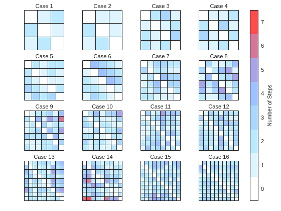
We immediately notice some inconsistencies, perhaps to be expected of the eccentric and cunning dictator. Things are pretty simple for the configurations with a small number of islands, but the minimum number of steps n can increase sharply and disproportionally to the additional number of islands. Cases 8 and 9 specifically have a particularly large n (relative to their grid dimensions), and case 14 has the largest n, almost double that of case 16 despite the fact that the latter has one extra island.
To visualize how this is possible, let's plot the path corresponding to the largest n for each case (though note that there might be multiple possible paths for each case):
figure
tiledlayout('flow','TileSpacing','tight','Padding','tight');
for i = plot_cases
nexttile
% Changing the layout to circular so we can better visualize the paths
p = plot(D{i},'ArrowSize',10,'Layout','Circle');
% Alternatively we could use the XData and YData properties if the positions of the islands were provided
axis([-1.5 1.5 -1.5 1.75])
[row,col] = ind2sub(size(d{i}),id(i));
highlight(p,shortestpath(D{i},row,col),'EdgeColor','r','NodeColor','r','LineWidth',2)
lims = axis;
text(lims(1)+diff(lims(1:2))*0.05,lims(3)+diff(lims(3:4))*0.9,sprintf('n = %d',d{i}(row,col)))
end
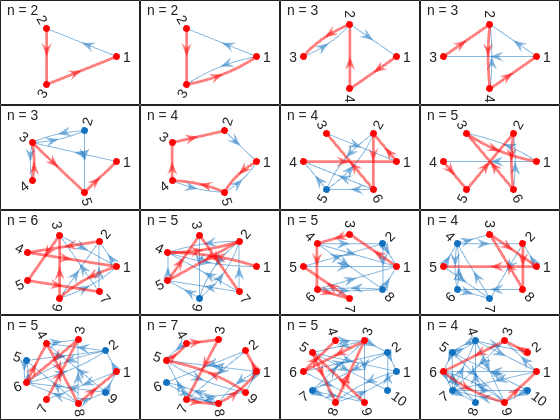
And busted! Unraveled! Exposed! Lord Ned has clearly been taking advantages of the tectonic forces by instructing his corrupt civil engineer lackeys to design the bridges to purposely force the visitors to go around in circles in order to drain them of their precious savings. In particular, for cases 8 and 9, he would have them go through every single island just to get from one island to another, whereas for case 14 they would have to visit 8 of the 9 islands just to get to their destination. If that's not diabolical then I don't know what is!
Ned jokes aside, I hope you enjoyed this contest just as much as I did, and that you found this article useful. I look forward to seeing more creative problems and solutions in the future.
I am deeply honored to announce the official publication of my latest academic volume:
MATLAB for Civil Engineers: From Basics to Advanced Applications
(Springer Nature, 2025).
This work serves as a comprehensive bridge between theoretical civil engineering principles and their practical implementation through MATLAB—a platform essential to the future of computational design, simulation, and optimization in our field.
Structured to serve both academic audiences and practicing engineers, this book progresses from foundational MATLAB programming concepts to highly specialized applications in structural analysis, geotechnical engineering, hydraulic modeling, and finite element methods. Whether you are a student building analytical fluency or a professional seeking computational precision, this volume offers an indispensable resource for mastering MATLAB's full potential in civil engineering contexts.
With rigorously structured examples, case studies, and research-aligned methods, MATLAB for Civil Engineers reflects the convergence of engineering logic with algorithmic innovation—equipping readers to address contemporary challenges with clarity, accuracy, and foresight.
📖 Ideal for:
— Graduate and postgraduate civil engineering students
— University instructors and lecturers seeking a structured teaching companion
— Professionals aiming to integrate MATLAB into complex real-world projects
If you are passionate about engineering resilience, data-informed design, or computational modeling, I invite you to explore the work and share it with your network.
🧠 Let us advance the discipline together through precision, programming, and purpose.

Hi everyone,
I've recently joined a forest protection team in Greece, where we use drones for various tasks. This has sparked my interest in drone programming, and I'd like to learn more about it. Can anyone recommend any beginner-friendly courses or programs that teach drone programming?
I'm particularly interested in courses that focus on practical applications and might align with the work we do in forest protection. Any suggestions or guidance would be greatly appreciated!
Thank you!