System Specification and Design | Developing Radio Applications for RFSoC with MATLAB & Simulink, Part 2
From the series: Developing Radio Applications for RFSoC with MATLAB and Simulink
System specifications for a range-Doppler radar are the driver for hardware/software implementation decisions when targeting SoC architectures like Xilinx® RFSoC devices.
In this second video in the series, see how specifications like peak bandwidth, range, and pulse rates serve as the basis for making implementation designs.
Review the process of frequency planning, which includes setting parameters such as intermediate frequency (IF), sampling rate (Fs), NCO mixer frequency, decimation/interpolation factor, and FPGA clock rate. Find out how to use simulation in Simulink® to validate the RF-ADC digital down conversation chain. Once the DDC chain is validated, learn how you can use the simulation of the complete system—with models of radar targets, range-Doppler radar processing, and detection—to determine whether targets are being detected. The resulting behavioral simulation model serves as the basis for hardware/software partitioning in Part 3 of this video series.
Published: 7 Jan 2021
In this video series, you'll learn how to use model based design approach to develop radio frequency applications for the Xilinx RFSoC platform. In the first video, we did a brief overview of RFSoC and introduced the hardware-software co-design methodology for implementing algorithms on system-on-chip devices. In part 2, we'll take a look at a real world application and develop a Range-Doppler radar system for RFSoC. We'll see how to take high level specifications and use that to make system level engineering decisions using modeling and simulation.
Let's take a look at our target application, Range-Doppler radar. Range-Doppler radar is a pulsed radar system used to estimate range and velocity of target objects. The range of an object is estimated using the returns from a single pulse, whereas the velocity is estimated by integrating multiple pulses over a coherent processing interval.
So for our system specifications for the Range-Doppler radar system we're designing, we need 200 megahertz of instantaneous bandwidth centered at x-band around 10 gigahertz. Our radar needs to estimate up to five kilometers of range at a maximum. And for velocity processing, we need to integrate up to 512 pulses per coherent processing interval.
Now, let's put our systems engineering hat on for a second. Look at some of the questions we're going to be thinking about as we go through this process from the top down. So first of all, what does the algorithm look like? What's the processing I need to implement to estimate the range and velocity?
What are the required data rates associated with that processing? From my algorithm, what part should be implemented in the programmable object versus what should be implemented in software? And as I evaluate this partitioning, what approach is going to have the best throughput, but also what approach would be the simplest to implement? So keep those in mind as we go through this process here.
And we start at systems specification for hardware-software co-design, and for RFSoC systems, the first thing we need to do here is some frequency planning. So our signal is at x-band, around 10 gigahertz, but the RFSoC data converters have a max input frequency of 4 gigahertz. So how do we go from RF to digital baseband and vise versa? Well, there's a number of parameters we're going to have to determine here, so let's take a look at the RF-ADC and its digital down conversion chain as specified in the Xilinx Product Guide 269.
So on the left side here represents our RF domain. On the right is our digital. We have our received signal coming in at an intermediate frequency, which is going to be produced with external RF hardware. We mix the 10 gigahertz signal down to something less than four gigahertz, so that it can be sampled by the RF-ADC.
We need to decide what frequency to run this data converter at, something less than about 4 gigasamples per second. And then we will configure the digital down conversion starting with the complex NCO and then the built-in decimators. And then finally, at the FPGA interface, we're going to pack up to 8 samples per clock cycle, so that will divide the sampling frequency down to an FPGA clock frequency.
One way to start this is by choosing the decimation factor based on our signal bandwidth. So we know, from our specifications, we need 200 megahertz of instantaneous bandwidth for the signal, and from that Product Guide 269, if we look at the decimation filters built into the down conversion chain, we have an 80% Nyquist pass band. So using that information, we can set up this little inequality here, and then let's just go ahead and choose decimation factor of 8. And so we plug that in, and that gets us to a sampling frequency of at least 2,000 megahertz or 2 gigahertz-- gigasamples per second.
Now, that ADC sampling frequency is going to be divided down by 8, the decimation, and that gets us to an effective sampling frequency of 250 samples per second. But we can choose to pack 2 samples per FPGA clock cycle so that the FPGA clock rate is 125 megahertz. So your FPGA guy will thank you. That will make their job a little easier in terms of meeting timing.
Further, we're going to choose an intermediate frequency of 2,500 megahertz so that when we sample it at 2 gigasamples per second, it's going to alias down from the third Nyquist zone to 500 megahertz. Then finally, we set our NCO frequency to negative 500 megahertz to move that signal down to baseband.
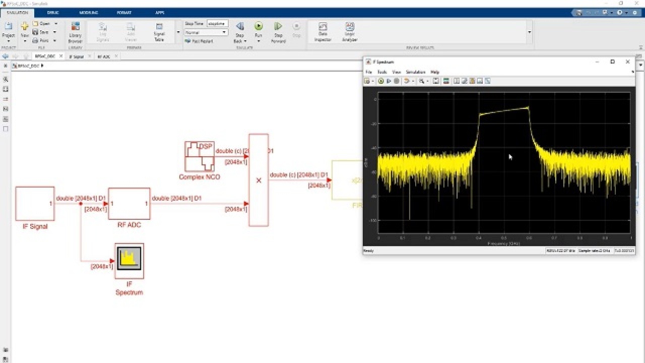
And we can actually simulate this whole process using Simulink. So I have a model here I built up of the digital down conversion chain for the RF-ADC, and you'll note that this has three stages of filters here. That's the way the 8x decimation is implemented, is with three stages of 2x decimation.
So we can run this, and so here in this view, this is our IF spectrum. This is the signal before it touches the ADC centered at 500 megahertz, and then after it gets mixed with negative 500 megahertz and then decimated down, open our baseband spectrum here, we have centered at 0. And look at our frequency range here. We have negative 125 megahertz to 125 megahertz, which is our effective FS of 250 megahertz divided by 2. There's our plus or minus FS over 2.
So all the parameters of this model are defined in a MATLAB script. That makes it easy to play with this. If we had different system level specifications, we could just plug this in here and then press Play and make sure that our signal ends up where we think it will in the baseband spectrum.
So the next step here is to implement the Range-Doppler algorithm using a high level behavioral system model, and the key word here is behavioral. We're not thinking about the hardware-software implementation. We just want to simulate our system at a high level, which will serve as our reference for the implementation later on. But we can build up a model for this also in Simulink, so I've got that right here.
So there's four subsystems here. We have the waveform generation. We have our target model. And if we dig in here, you see this is actually a model reference, so it's a separate model, which means I can reuse it inside of other top level models.
And what we're doing here is actually simulating the RF domain, our channel out to, in this case here, two targets we're simulating-- transmit channel and then receive path back to the receiver here. And notice if we plug in to this block here, specify the carrier frequency FC, which maps back to my x-band specification of 10 gigahertz. So we're, again, simulating here the RF domain, and then inside here is where we get into the digital domain and the algorithm implementation. Here's a Range-Doppler response block that we're feeding our collection of pulses into, and we're going to feed, finally, this into a detection algorithm, which is a 2DC fly.
So we can run this, and we'll get some nice visual results here as this guy runs. So there's our two targets-- one at 3 kilometers and negative 100 meters per second. The other one at 4 kilometers, 150 meters per second. So the left input here is just our Range-Doppler processing output, and then on the right is a binary detection map where we're determining, for each of these pixels here, whether we think that represents a target or not.
And so again, the value of this model here is we can figure out all of our radar parameters, things like PRF, how much power we need at the transmitter, things like that, all stuff that should be figured out well before we get into the hardware-software implementation details. This concludes part 2 the video series. In part 3, we'll continue with the Range-Doppler radar example and evaluate different hardware-software partitioning strategies using a mix of simulation and hardware profiling based analysis.
Related Products
Learn More


Select a Web Site
Choose a web site to get translated content where available and see local events and offers. Based on your location, we recommend that you select: United States.
You can also select a web site from the following list
Americas
- América Latina (Español)
- Canada (English)
- United States (English)
Europe
- Belgium (English)
- Denmark (English)
- Deutschland (Deutsch)
- España (Español)
- Finland (English)
- France (Français)
- Ireland (English)
- Italia (Italiano)
- Luxembourg (English)
- Netherlands (English)
- Norway (English)
- Österreich (Deutsch)
- Portugal (English)
- Sweden (English)
- Switzerland
- United Kingdom (English)