phased.RangeEstimator
Range estimation
Description
The phased.RangeEstimator
System object™ estimates the ranges of targets. Input to the estimator consists of a
range-response or range-Doppler response data cube, and detection locations from a
detector. When information about clusters of detections is available, the ranges are
computed using cluster information. Clustering associates multiple detections into one
extended detection.
To compute the detections for a range-response or range-Doppler cube:
Create the
phased.RangeEstimatorobject and set its properties.Call the object with arguments, as if it were a function.
To learn more about how System objects work, see What Are System Objects?
Creation
Description
estimator = phased.RangeEstimator creates a range
estimator System object, estimator.
estimator = phased.RangeEstimator(
creates a System object, Name=Value)estimator, with each specified property
Name set to the specified Value. You
can specify additional name and value arguments in any order as
(Name1=Value1,...,NameN=ValueN).
Properties
Usage
Syntax
Description
You can combine optional input and output arguments when their enabling
properties are set. Optional inputs and outputs must be listed in the same order
as the order of the enabling properties. For example,
[.rngest,rngvar]
= estimator(resp,rnggrid,detidx,noisepower,clusterids)
Note
The object performs an initialization the first time the object is executed. This
initialization locks nontunable properties
and input specifications, such as dimensions, complexity, and data type of the input data.
If you change a nontunable property or an input specification, the System object issues an error. To change nontunable properties or inputs, you must first
call the release method to unlock the object.
Input Arguments
Output Arguments
Object Functions
To use an object function, specify the
System object as the first input argument. For
example, to release system resources of a System object named obj, use
this syntax:
release(obj)
Examples
To estimate the range and speed of three targets, create a range-Doppler map using the phased.RangeDopplerResponse System object™. Then use the phased.RangeEstimator and phased.DopplerEstimator System objects to estimate range and speed. The transmitter and receiver are collocated isotropic antenna elements forming a monostatic radar system.
The transmitted signal is a linear FM waveform with a pulse repetition interval (PRI) of 7.0 μs and a duty cycle of 2%. The operating frequency is 77 GHz and the sample rate is 150 MHz.
fs = 150e6;
c = physconst("LightSpeed");
fc = 77.0e9;
pri = 7e-6;
prf = 1/pri;
Set up the scenario parameters. The transmitter and receiver are stationary and located at the origin. The targets are 500, 530, and 750 meters from the radar along the x-axis. The targets move along the x-axis at speeds of –60, 20, and 40 m/s. All three targets have a nonfluctuating radar cross-section (RCS) of 10 dB. Create the target and radar platforms.
Numtgts = 3;
tgtpos = zeros(Numtgts);
tgtpos(1,:) = [500 530 750];
tgtvel = zeros(3,Numtgts);
tgtvel(1,:) = [-60 20 40];
tgtrcs = db2pow(10)*[1 1 1];
tgtmotion = phased.Platform(tgtpos,tgtvel);
target = phased.RadarTarget(PropagationSpeed=c,OperatingFrequency=fc, ...
    MeanRCS=tgtrcs);
radarpos = [0;0;0];
radarvel = [0;0;0];
radarmotion = phased.Platform(radarpos,radarvel);
Create the transmitter and receiver antennas.
txantenna = phased.IsotropicAntennaElement;
rxantenna = clone(txantenna);
Set up the transmitter-end signal processing. Create an upsweep linear FM signal with a bandwidth of one half the sample rate. Find the length of the PRI in samples and then estimate the rms bandwidth and range resolution.
bw = fs/2;
waveform = phased.LinearFMWaveform(SampleRate=fs, ...
    PRF=prf,OutputFormat="Pulses",NumPulses=1,SweepBandwidth=fs/2, ...
    DurationSpecification="Duty cycle",DutyCycle=0.02);
sig = waveform();
Nr = length(sig);
bwrms = bandwidth(waveform)/sqrt(12);
rngrms = c/bwrms;
Set up the transmitter and radiator System object properties. The peak output power is 10 W and the transmitter gain is 36 dB.
peakpower = 10;
txgain = 36.0;
transmitter = phased.Transmitter( ...
    PeakPower=peakpower, ...
    Gain=txgain, ...
    InUseOutputPort=true);
radiator = phased.Radiator( ...
    Sensor=txantenna,...
    PropagationSpeed=c,...
    OperatingFrequency=fc);
Set up the free-space channel in two-way propagation mode.
channel = phased.FreeSpace( ...
    SampleRate=fs, ...
    PropagationSpeed=c, ...
    OperatingFrequency=fc, ...
    TwoWayPropagation=true);
Set up the receiver-end processing. Set the receiver gain and noise figure.
collector = phased.Collector( ...
    Sensor=rxantenna, ...
    PropagationSpeed=c, ...
    OperatingFrequency=fc);
rxgain = 42.0;
noisefig = 1;
receiver = phased.ReceiverPreamp( ...
    SampleRate=fs, ...
    Gain=rxgain, ...
    NoiseFigure=noisefig);
Loop over the pulses to create a data cube of 128 pulses. For each step of the loop, move the target and propagate the signal. Then put the received signal into the data cube. The data cube contains the received signal per pulse. Ordinarily, a data cube has three dimensions where the last dimension corresponds to antennas or beams. Because only one sensor is used, the cube has only two dimensions.
The processing steps are:
Move the radar and targets.
Transmit a waveform.
Propagate the waveform signal to the target.
Reflect the signal from the target.
Propagate the waveform back to the radar. Two-way propagation enables you to combine the return propagation with the outbound propagation.
Receive the signal at the radar.
Load the signal into the data cube.
Np = 128;
dt = pri;
cube = zeros(Nr,Np);
for n = 1:Np
    [sensorpos,sensorvel] = radarmotion(dt);
    [tgtpos,tgtvel] = tgtmotion(dt);
    [tgtrng,tgtang] = rangeangle(tgtpos,sensorpos);
    sig = waveform();
    [txsig,txstatus] = transmitter(sig);
    txsig = radiator(txsig,tgtang);
    txsig = channel(txsig,sensorpos,tgtpos,sensorvel,tgtvel);
    tgtsig = target(txsig);
    rxcol = collector(tgtsig,tgtang);
    rxsig = receiver(rxcol);
    cube(:,n) = rxsig;
end
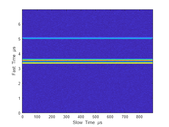
Display the data cube containing signals per pulse.
imagesc([0:(Np-1)]*pri*1e6,[0:(Nr-1)]/fs*1e6,abs(cube))
xlabel("Slow Time {\mu}s")
ylabel("Fast Time {\mu}s")
axis xy
Create and display the range-Doppler image for 128 Doppler bins. The image shows range vertically and speed horizontally. Use the linear FM waveform for match filtering. The image is here is the range-Doppler map.
ndop = 128;
rangedopresp = phased.RangeDopplerResponse(SampleRate=fs, ...
    PropagationSpeed=c,DopplerFFTLengthSource="Property", ...
    DopplerFFTLength=ndop,DopplerOutput="Speed", ...
    OperatingFrequency=fc);
matchingcoeff = getMatchedFilter(waveform);
[rngdopresp,rnggrid,dopgrid] = rangedopresp(cube,matchingcoeff);
imagesc(dopgrid,rnggrid,10*log10(abs(rngdopresp)))
xlabel("Closing Speed (m/s)")
ylabel("Range (m)")
axis xy
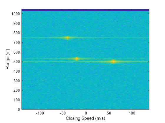
Because the targets lie along the positive x-axis, positive velocity in the global coordinate system corresponds to negative closing speed. Negative velocity in the global coordinate system corresponds to positive closing speed.
Estimate the noise power after matched filtering. Create a constant noise background image for simulation purposes.
mfgain = matchingcoeff'*matchingcoeff;
dopgain = Np;
noisebw = fs;
noisepower = noisepow(noisebw,receiver.NoiseFigure,receiver.ReferenceTemperature);
noisepowerprc = mfgain*dopgain*noisepower;
noise = noisepowerprc*ones(size(rngdopresp));
Create the range and Doppler estimator objects.
rangeestimator = phased.RangeEstimator(NumEstimatesSource="Auto", ...
    VarianceOutputPort=true,NoisePowerSource="Input port", ...
    RMSResolution=rngrms);
dopestimator = phased.DopplerEstimator(VarianceOutputPort=true, ...
    NoisePowerSource="Input port",NumPulses=Np);
Locate the target indices in the range-Doppler image. Instead of using a CFAR detector, for simplicity, use the known locations and speeds of the targets to obtain the corresponding index in the range-Doppler image.
detidx = NaN(2,Numtgts);
tgtrng = rangeangle(tgtpos,radarpos);
tgtspd = radialspeed(tgtpos,tgtvel,radarpos,radarvel);
tgtdop = 2*speed2dop(tgtspd,c/fc);
for m = 1:numel(tgtrng)
    [~,iMin] = min(abs(rnggrid-tgtrng(m)));
    detidx(1,m) = iMin;
    [~,iMin] = min(abs(dopgrid-tgtspd(m)));
    detidx(2,m) = iMin;
end
Find the noise power at the detection locations.
ind = sub2ind(size(noise),detidx(1,:),detidx(2,:));
Estimate the range and range variance at the detection locations. The estimated ranges agree with the postulated ranges.
[rngest,rngvar] = rangeestimator(rngdopresp,rnggrid,detidx,noise(ind))
rngest = 3×1

  499.7911
  529.8380
  750.0983
rngvar = 3×1
10-4 ×

    0.0273
    0.0276
    0.2094
Estimate the speed and speed variance at the detection locations. The estimated speeds agree with the predicted speeds.
[spdest,spdvar] = dopestimator(rngdopresp,dopgrid,detidx,noise(ind))
spdest = 3×1

   60.5241
  -19.6167
  -39.5838
spdvar = 3×1
10-5 ×

    0.0806
    0.0816
    0.6188
More About
Algorithms
References
[1] Richards, M. Fundamentals of Radar Signal Processing. 2nd ed. McGraw-Hill Professional Engineering, 2014.
[2] Richards, M., J. Scheer, and W. Holm. Principles of Modern Radar: Basic Principles. SciTech Publishing, 2010.
Extended Capabilities
Version History
Introduced in R2017a
See Also
Functions
Objects
phased.DopplerEstimator|phased.RangeResponse|phased.RangeDopplerResponse|phased.CFARDetector|phased.CFARDetector2D