clusterDBSCAN
Density-based algorithm for clustering data
Description
clusterDBSCAN clusters data points belonging to a
P-dimensional feature space using the density-based spatial clustering of
applications with noise (DBSCAN) algorithm. The clustering algorithm assigns points that are
close to each other in feature space to a single cluster. For example, a radar system can
return multiple detections of an extended target that are closely spaced in range, angle, and
Doppler. clusterDBSCAN assigns these detections to a single detection.
The DBSCAN algorithm assumes that clusters are dense regions in data space separated by regions of lower density and that all dense regions have similar densities.
To measure density at a point, the algorithm counts the number of data points in a neighborhood of the point. A neighborhood is a P-dimensional ellipse (hyperellipse) in the feature space. The radii of the ellipse are defined by the P-vector ε. ε can be a scalar, in which case, the hyperellipse becomes a hypersphere. Distances between points in feature space are calculated using the Euclidean distance metric. The neighborhood is called an ε-neighborhood. The value of ε is defined by the
Epsilonproperty.Epsiloncan either be a scalar or P-vector:A vector is used when different dimensions in feature space have different units.
A scalar applies the same value to all dimensions.
Clustering starts by finding all core points. If a point has a sufficient number of points in its ε-neighborhood, the point is called a core point. The minimum number of points required for a point to become a core point is set by the
MinNumPointsproperty.The remaining points in the ε-neighborhood of a core point can be core points themselves. If not, they are border points. All points in the ε-neighborhood are called directly density reachable from the core point.
If the ε-neighborhood of a core point contains other core points, the points in the ε-neighborhoods of all the core points merge together to form a union of ε-neighborhoods. This process continues until no more core points can be added.
All points in the union of ε-neighborhoods are density reachable from the first core point. In fact, all points in the union are density reachable from all core points in the union.
All points in the union of ε-neighborhoods are also termed density connected even though border points are not necessarily reachable from each other. A cluster is a maximal set of density-connected points and can have an arbitrary shape.
Points that are not core or border points are noise points. They do not belong to any cluster.
The
clusterDBSCANobject can estimate ε using a k-nearest neighbor search, or you can specify values. To let the object estimate ε, set theEpsilonSourceproperty to'Auto'.The
clusterDBSCANobject can disambiguate data containing ambiguities. Range and Doppler are examples of possibly ambiguous data. SetEnableDisambiguationproperty totrueto disambiguate data.
To cluster detections:
Create the
clusterDBSCANobject and set its properties.Call the object with arguments, as if it were a function.
To learn more about how System objects work, see What Are System Objects?
Creation
Description
clusterer = clusterDBSCANclusterDBSCAN object, clusterer, with default
property values.
clusterer = clusterDBSCAN(Name,Value)clusterDBSCAN object, clusterer, with each
specified Property
Name set to the corresponding Value. You can
specify additional pairs of arguments in any order as
Name1=Value1,...,NameN=ValueN. Any unspecified
properties take default values. For example,
clusterer = clusterDBSCAN(MinNumPoints=3,Epsilon=2, ...
EnableDisambiguation=true,AmbiguousDimension=[1 2]);clusterer object with the EnableDisambiguation
property set to true and the AmbiguousDimension set to
[1,2].Properties
Usage
Syntax
Description
[
also returns an alternate set of cluster IDs, idx,clusterids] = clusterer(X)clusterids, for use in
the phased.RangeEstimator and phased.DopplerEstimator objects. clusterids assigns a
unique ID to each noise point.
[___] = clusterer(
automatically estimates epsilon from the input data matrix, X,update)X, when
update is set to true. The estimation uses a
k-NN search to create a set of search curves. For more information,
see Estimate Epsilon. The estimate is an
average of the L most recent Epsilon values where L
is specified in EpsilonHistoryLength
To enable this syntax, set the EpsilonSource property to
'Auto', optionally set the MaxNumPoints
property, and also optionally set the EpsilonHistoryLength
property.
Input Arguments
Output Arguments
Object Functions
To use an object function, specify the
System object™ as the first input argument. For
example, to release system resources of a System object named obj, use
this syntax:
release(obj)
Examples
Create detections of extended objects with measurements in range and Doppler. Assume the maximum unambiguous range is 20 m and the unambiguous Doppler span extends from Hz to Hz. Data for this example is contained in the dataClusterDBSCAN.mat file. The first column of the data matrix represents range, and the second column represents Doppler.
The input data contains the following extended targets and false alarms:
an unambiguous target located at
an ambiguous target in Doppler located at
an ambiguous target in range located at
an ambiguous target in range and Doppler located at
5 false alarms
Create a clusterDBSCAN object and specify that disambiguation is not performed by setting EnableDisambiguation to false. Solve for the cluster indices.
load('dataClusterDBSCAN.mat');
cluster1 = clusterDBSCAN('MinNumPoints',3,'Epsilon',2, ...
    'EnableDisambiguation',false);
idx = cluster1(x);
Use the clusterDBSCAN plot object function to display the clusters.
plot(cluster1,x,idx)
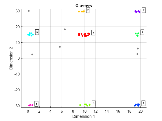
The plot indicates that there are eight apparent clusters and six noise points. The 'Dimension 1' label corresponds to range and the 'Dimension 2' label corresponds to Doppler.
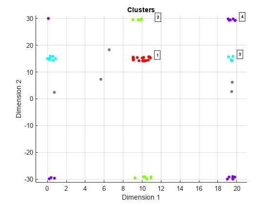
Next, create another clusterDBSCAN object and set EnableDisambiguation to true to specify that clustering is performed across the range and Doppler ambiguity boundaries.
cluster2 = clusterDBSCAN('MinNumPoints',3,'Epsilon',2, ...
    'EnableDisambiguation',true,'AmbiguousDimension',[1 2]);
Perform the clustering using ambiguity limits and then plot the clustering results. The DBSCAN clustering results correctly show four clusters and five noise points. For example, the points at ranges close to zero are clustered with points near 20 m because the maximum unambiguous range is 20 m.
amblims = [0 maxRange; minDoppler maxDoppler];
idx = cluster2(x,amblims);
plot(cluster2,x,idx)
Cluster two-dimensional Cartesian position data using clusterDBSCAN. To illustrate how the choice of epsilon affects clustering, compare the results of clustering with Epsilon set to 1 and Epsilon set to 3.
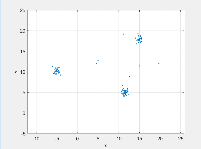
Create random target position data in xy Cartesian coordinates.
x = [rand(20,2)+12; rand(20,2)+10; rand(20,2)+15];
plot(x(:,1),x(:,2),'.')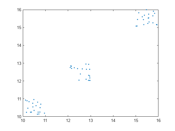
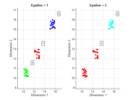
Create a clusterDBSCAN object with the Epsilon property set to 1 and the MinNumPoints property set to 3.
clusterer = clusterDBSCAN('Epsilon',1,'MinNumPoints',3);
Cluster the data when Epsilon equals 1.
idxEpsilon1 = clusterer(x);
Cluster the data again but with Epsilon set to 3. You can change the value of Epsilon because it is a tunable property.
clusterer.Epsilon = 3;
idxEpsilon2 = clusterer(x);
Plot the clustering results side-by-side. Do this by passing in the axes handles and titles into the plot method. The plot shows that for Epsilon set to 1, three clusters appear. When Epsilon is 3, the two lower clusters are merged into one.
hAx1 = subplot(1,2,1);
plot(clusterer,x,idxEpsilon1, ...
    'Parent',hAx1,'Title','Epsilon = 1')
hAx2 = subplot(1,2,2);
plot(clusterer,x,idxEpsilon2, ...
    'Parent',hAx2,'Title','Epsilon = 3')
Algorithms
This section illustrates the basic principles of cluster formation. The figure shows points in a two-dimensional feature space. The clusters are compact and well-separated. A few noise points appear.
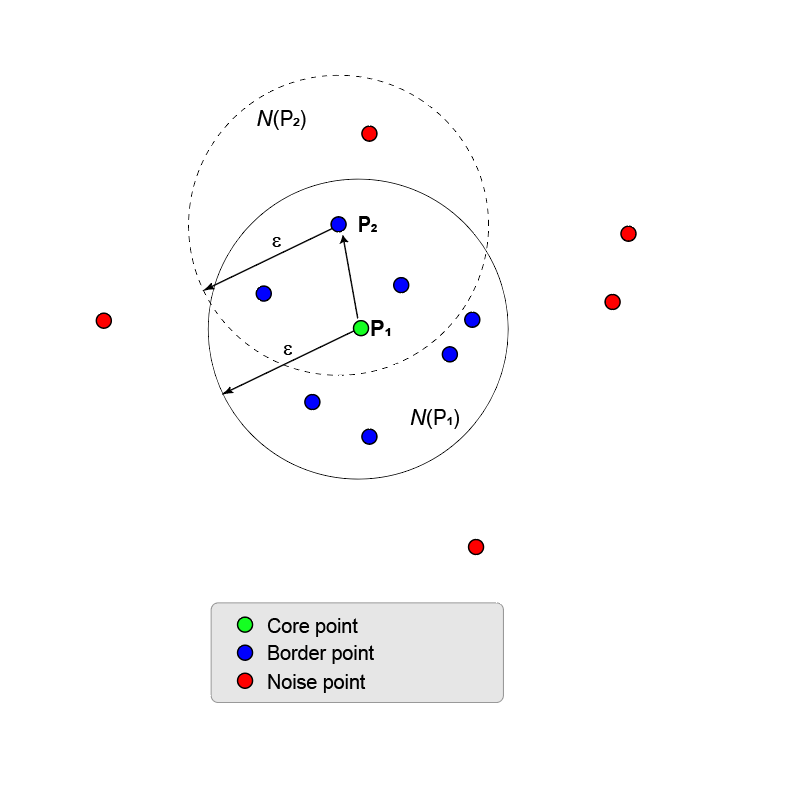
Clusters start from core points. The first step in the algorithm is identifying all core points.
The figure here shows the point P1 and its ε-neighborhood Nε(P1). The ε-neighborhood has eight points (including itself) within a radius ε. Using the
MinNumPointsproperty to set the threshold to 8 means that P1 is a core point. The blue points that lie within Nε are called border points. These border points are directly density reachable from the core point P1.No other points in the figure have enough neighboring points in their ε-neighborhood to become a core point. P2 is not a core point because it has only five points within its neighborhood. P2 is directly density reachable from P1. The reverse is not true because P2 is not a core point. The one-way arrow connecting the two points shows this asymmetry.
Points that fall outside Nε(P1) are noise points (red) and do not belong to the cluster.
Because no other points are core points, the core point and border points are a maximal set of density-connected points and therefore form a cluster.
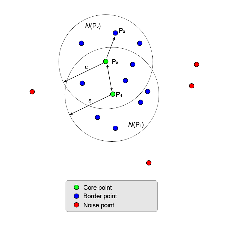
The next figure shows a larger set of points containing two core points, P1 and P2. P2 is a border point of P1 but P2 also has enough points in its own neighborhood to become a core point. Because they are both core points, P1 is directly density reachable from P2, and P1 is directly density reachable from P2. The two-way arrow connecting them shows this symmetry.
P3 is directly density reachable from P2 but not from P1 (as indicated by the one-way arrow). However, P3 is called simply density reachable from P1.
Because no other points are core points, the two core points and their border points form a maximal set of density-connected points and form one cluster.
This process of growing a cluster can be extended from core point to core point until there are no more core points to add. The core points and the border points belong to the same cluster. In general, a point Pn is density reachable from point P1 when there is a chain of core points, P1,P2, P3, …, Pn-1 such that each core point Pi+1 is directly density reachable from Pi, and Pn is directly density reachable from Pn-1.
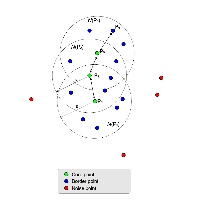
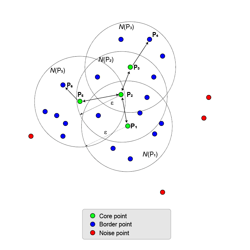
The next figure illustrates some properties of density connectivity.
A cluster can have multiple branching chains, for example (P1, P2, P3, P4) and (P1, P2, P5, P6).
Two points, P6 and P4, are density connected when there is a third point P2 such that P6 and P4 are density reachable from P2.
Two density connected points are not necessarily density reachable from one another.
A maximal set of density connected points define a cluster. It does not matter which core point is the starting core point.
All points in a cluster are density reachable from all core points.
DBSCAN clustering requires a value for the neighborhood size parameter ε. The
clusterDBSCAN object and the
clusterDBSCAN.estimateEpsilon function use a
k-nearest-neighbor search to estimate a scalar epsilon. Let
D be the distance of any point P to its
kth nearest neighbor. Define a
Dk(P)-neighborhood as a
neighborhood surrounding P that contains its
k-nearest neighbors. There are k + 1 points in the
Dk(P)-neighborhood
including the point P itself. An outline of the estimation algorithm
is:
For each point, find all the points in its Dk(P)-neighborhood
Accumulate the distances in all Dk(P)-neighborhoods for all points into a single vector.
Sort the vector by increasing distance.
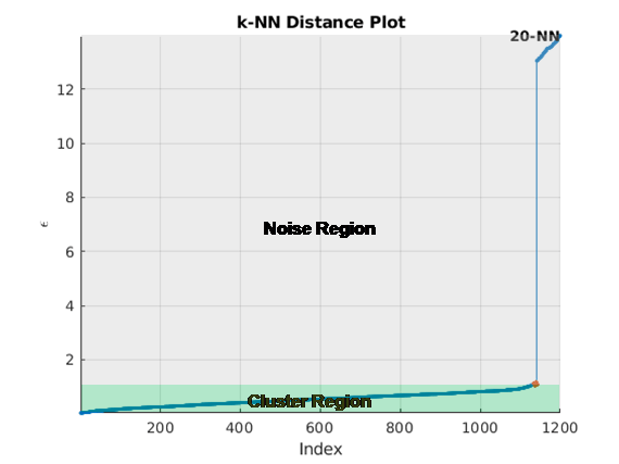
Plot the sorted k-dist graph, which is the sorted distance against point number.
Find the knee of the curve. The value of the distance at that point is an estimate of epsilon.
The figure here shows distance plotted against point index for k = 20. The knee occurs at approximately 1.5. Any points below this threshold belong to a cluster. Any points above this value are noise.
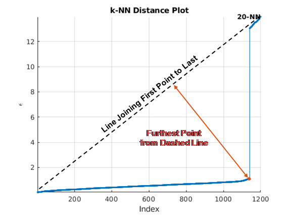
There are several methods to find the knee of the curve. clusterDBSCAN and
clusterDBSCAN.estimateEpsilon first define the line connecting the
first and last points of the curve. The ordinate of the point on the sorted
k-dist graph furthest from the line and perpendicular to the line
defines epsilon.
When you specify a range of k values, the algorithm averages the estimate epsilon values for all curves. This figure shows that epsilon is fairly insensitive to k for k ranging from 14 through 19.
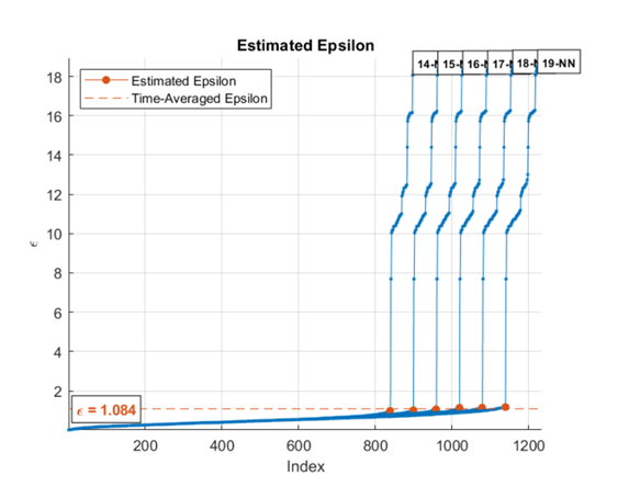
To create a single k-NN distance graph, set the
MinNumPoints property equal to the
MaxNumPoints property.
References
[1] Ester M., Kriegel H.-P., Sander J., and Xu X. "A Density-Based Algorithm for Discovering Clusters in Large Spatial Databases with Noise". Proc. 2nd Int. Conf. on Knowledge Discovery and Data Mining, Portland, OR, AAAI Press, 1996, pp. 226-231.
[2] Erich Schubert, Jörg Sander, Martin Ester, Hans-Peter Kriegel, and Xiaowei Xu. 2017. "DBSCAN Revisited, Revisited: Why and How You Should (Still) Use DBSCAN". ACM Trans. Database Syst. 42, 3, Article 19 (July 2017), 21 pages.
[3] Dominik Kellner, Jens Klappstein and Klaus Dietmayer, "Grid-Based DBSCAN for Clustering Extended Objects in Radar Data", 2012 IEEE Intelligent Vehicles Symposium.
[4] Thomas Wagner, Reinhard Feger, and Andreas Stelzer, "A Fast Grid-Based Clustering Algorithm for Range/Doppler/DoA Measurements", Proceedings of the 13th European Radar Conference.
[5] Mihael Ankerst, Markus M. Breunig, Hans-Peter Kriegel, Jörg Sander, "OPTICS: Ordering Points To Identify the Clustering Structure", Proc. ACM SIGMOD’99 Int. Conf. on Management of Data, Philadelphia PA, 1999.
Extended Capabilities
Version History
Introduced in R2021a