Why Solving Classification Using Reinforcement Learning Is Not Recommended

This example shows how to solve a regression problem using both a supervised learning approach and a reinforcement learning approach, illustrating the differences between these methods. This example also illustrates why reinforcement learning is not the right tool to solve a supervised learning problem. For more information on the relationship between reinforcement and supervised learning, see [1].

Introduction

The problem considered in this example is the classification of images containing handwritten digits. In a supervised learning setting, you solve the problem by training a network to predict the known correct digit associated with each image in a training dataset. You then use images in a validation dataset to check how well the network is able to predict the correct digit given an unseen input image. For an example, see Create Simple Image Classification Network.

Similarly, in a reinforcement learning setting, you train an agent to predict the correct digit a associated with each image in the training dataset. Specifically, the agent's observation input is an image in the dataset, while the agent's action output is the predicted digit for the image. The environment then supplies to the agent a scalar reward that represents the quality of the agent prediction. Note that the reward only captures the information of whether the prediction was correct, but does not capture the full information of which one is the right digit for the presented image. By contrast, the right digit information is fully used in the supervised learning setting, (which is why training is generally much faster for supervised learning).

Because the next observation is independent on the action, this type of reinforcement learning problem can be classified as a "contextual bandit" problem. In these problems, the environment has no state dynamics, so the reward is only influenced by the current observation and action.

The following figure shows how contextual bandit problems are special cases of reinforcement learning problems.

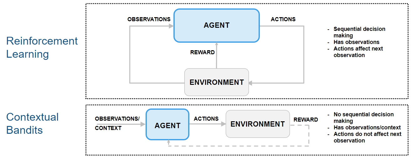
For an example on how to use an agent to solve a contextual bandit problem, see Train Reinforcement Learning Agent for Simple Contextual Bandit Problem. For an example discussing regression as a contextual bandit problem, see Why Solving Regression Using Reinforcement Learning is Not Recommended. For a comprehensive introduction to bandit problems, see [2].

Preserve Random Number Sequence for Reproducibility

Some sections in this example require random number computations. Specify the seed and random number generator algorithm at the beginning of a section to use the same random number sequence each time you run it. Preserving the random number sequence allows you to reproduce the results of the section. For more information, see Results Reproducibility.

Set the random number seed to 0 and the algorithm to Mersenne Twister. For more information, see rng.

previousRngState = rng(0,"twister");

The output previousRngState is a structure that contains information about the previous state of the sequence. You will restore the state at the end of the example.

Extract Image Data and Create Training and Validation Sets

For this example, use the same digit data file in used in Create Simple Image Classification Network.

Unzip the digit sample data, unless the data folder already exists.

if ~exist("DigitsData","dir")
    unzip("DigitsData.zip")
end

Create an image datastore. The imageDatastore function automatically labels the images based on folder names. For more information about datastores, see Getting Started with Datastore.

imds = imageDatastore("DigitsData", ...
    IncludeSubfolders=true, ...
    LabelSource="foldernames");

Divide the data into training and validation data sets, so that each category in the training set contains 750 images and the validation set contains the remaining images from each label. splitEachLabel splits the image datastore into two new datastores for training and validation. Because there are 10 categories (one for each digit) the training datastore contains a total of 750*10 = 7500 available images.

numTrainFiles = 750;
[imdsTrain,imdsValidation] = ....
    splitEachLabel(imds,numTrainFiles,"randomized");

To view the class names, run the following command.

classNames = categories(imdsTrain.Labels)

Display a random image from the training datastore.

image(readimage(imdsTrain,randi(numTrainFiles*10)));
axis("square")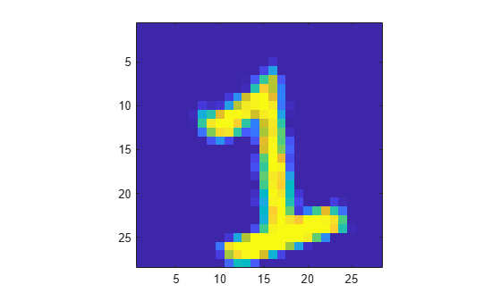

Create Custom Discrete-Action-Space Environment Object

Create the environment specifications. The (continuous) observation is a gray scale 28-by-28 pixels image, with each element normalized between 0 and 1, and the (discrete) action is the predicted digit (from 0 to 9) associated with the input image.

obsInfo = rlNumericSpec([28 28], ...
    LowerLimit=0, ...
    UpperLimit=1);
actInfo = rlFiniteSetSpec(0:9);

At the beginning of each training or simulation episode, a reset function resets the environment to an initial state and returns both the initial state (needed for the next environment step) and the resulting initial observation value (for the agent to see).

Display the custom reset function, which is provided in the file clsfResetFcn.m.

type("clsfResetFcn.m")

function [obs,x] = clsfResetFcn(imds,nmax)
% Reset function to set environment in random initial state.

% Read a random image from dataset, the image is the observation.
[obs,info] = readimage(imds,randi(nmax)); 

% Normalize image.
obs = double(obs)./255;

% State is the true label (used to calculate the reward).
x = grp2idx(info.Label)-1;

end

This function takes as input argument an image datastore (it could be either the training or validation set) and the total number of images in the dataset. The function then reads a random image, converts the image to a double, and normalizes it. The output arguments are the initial observation for the agent, (which is the normalized image), and the initial state of the environment, which is the correct label (0 to 9) associated with the image.

A step function is called by train (or sim) at each step of the training (or simulation) episode to advance the environment to the next step.

Display the custom step function, which is provided in the file clsfStepFcn.m.

type("clsfStepFcn.m")

function [nextObs,r,isdn,xp] = clsfStepFcn(a,x,imds,nmax)
% Custom step function to advance custom environment by one step.

% Calculate reward (reward for a).
r = double(a==x);

% Calculate next observation and state.

% Read a random image from dataset, the image is the next observation.
[nextObs,info] = readimage(imds,randi(nmax));

% Normalize image.
nextObs = double(nextObs)./255;

% Store new label (for use at the next step).
xp = grp2idx(info.Label)-1;

% Episode does not end because of an action.
isdn = 0;

end

This function takes as input arguments the action from the agent, the current environment state, an image datastore and the total number of images in the dataset.

First, the function calculates a reward for the agent, which is equal to one if the action is equal to the current state (this means the agent was able to correctly identify the image), and zero otherwise. Note that, differently from a supervised learning setting, when the guess is not correct, the environment does not convey to the agent any information about which label is the correct one.

The step function then reads a new random image, converts the image to a double, and normalizes it. The output arguments are the next observation for the agent, (which is the new normalized image), the reward associated with the agent action, an is-done flag that indicates if the episode is finished and the updated state of the environment, which is the correct label (0 to 9) associated with the new image.

Create the custom function environment object for training, using the training datastore.

Because the custom reset and step functions that you must pass to rlFunctionEnv must have exactly zero and two arguments, respectively, define the actual reset and step functions as anonymous functions (with zero and two arguments, respectively). In turn, these anonymous functions, call clsfResetFcn and clsfStepFcn, passing the additional imds and nmax arguments which are stored in the workspace of the anonymous function at definition time.

envTrain = rlFunctionEnv(obsInfo,actInfo, ...
    @(a,x) clsfStepFcn(a,x,imdsTrain,numTrainFiles*10), ...
    @() clsfResetFcn(imdsTrain,numTrainFiles*10));

For a more detailed example on custom step and reset functions, see Create Custom Environment Using Step and Reset Functions.

Create Discrete Categorical Actor from Custom Network

Policy gradient agents use a parameterized stochastic policy, which for discrete action spaces is implemented by a discrete categorical actor. This actor takes an observation as input and returns as output a random action sampled (among the finite number of possible actions) from a categorical probability distribution.

To model the parameterized policy within the actor, use a neural network with one input layer (which receives the content of the environment observation channel, as specified by obsInfo) and one output layer. The output layer must return a vector of probabilities for each possible action, as specified by actInfo.

Define the network as an array of layer objects. This is the same network used in the example Create Simple Image Classification Network.

layers = [
    imageInputLayer([28 28 1])
    convolution2dLayer(5,20)
    reluLayer
    fullyConnectedLayer(10)
    softmaxLayer
    ];

For more information about deep learning layers, see List of Deep Learning Layers.

The network is initialized randomly. Specify random seed and algorithm for reproducibility.

rng(0,"twister")

Create dlnetwork object.

net = dlnetwork(layers);

Display the number of learnable parameters.

summary(net)

   Initialized: true

   Number of learnables: 115.7k

   Inputs:
      1   'imageinput'   28×28×1 images

Create a discrete categorical actor, for more information, see rlDiscreteCategoricalActor.

actor = rlDiscreteCategoricalActor(net,obsInfo,actInfo);

To check your actor, use the getAction function to return a batch of 5 actions from a batch of 5 random observations, given the current network weights.

obs = rand([obsInfo.Dimension 5]);
act = getAction(actor,{obs});

Return the third element of the batch.

act{1}(1,1,3)

ans = 
3

To return the probability distribution of the actions, given an observation, use evaluate.

prb = evaluate(actor,{obs});
prb{1}(:,3)

ans = 10×1 single column vector

    0.1217
    0.0974
    0.0738
    0.1123
    0.1247
    0.0926
    0.1036
    0.1188
    0.0734
    0.0817

Create a PG Agent and Specify Agent Options

Create a rlPGAgent object using the previously created actor.

pgAgent = rlPGAgent(actor);

Set a lower learning rate and gradient thresholds to avoid instability.

pgAgent.AgentOptions.ActorOptimizerOptions.LearnRate = 1e-3;
pgAgent.AgentOptions.ActorOptimizerOptions.GradientThreshold = 1;

Because future reward is independent on the action, set a discount factor of zero.

pgAgent.AgentOptions.DiscountFactor = 0;

Configure Training Options

Create an evaluator object to evaluate the agent five times without exploration every 100 episodes.

evl = rlEvaluator(NumEpisodes=5,EvaluationFrequency=100);

Create a training options object. For more information on training options, see rlTrainingOptions.

trainOpts = rlTrainingOptions;

• Set the maximum number of steps per episode to 100 (note that the environment has no terminal state).

• Stop the training when the average reward collected over the evaluation episodes reaches 90. This means the agent can classify images with a 90% accuracy.

• In any case, stop after 5000 episodes (which is enough for the agent to see the same image approximately 100*5000/7500 = 66.6 times).

trainOpts.MaxEpisodes = 5000;
trainOpts.MaxStepsPerEpisode = 100;
trainOpts.StopTrainingCriteria = "EvaluationStatistic";
trainOpts.StopTrainingValue = 90;

Alternatively, because the next state is independent of the action, you can set the maximum number of steps per episode to 1 (and consequently allow for a larger number of episodes). Adopting this view, each episode is a stand-alone event in which the agent associates a single observation to a single action, that is, each episode represents an instance of a bandit problem with a different context (a different input value). You must use this approach if your environment does not allow multiple steps per episode.

However, if you use this alternative approach to train agents like PG agents, which calculate network gradients at the end of the episode and use only the steps available in the episode, then the network gradients are calculated using only a single observation and reward. This can lead to inefficient or unstable learning.

For an example using this alternative approach, see Train Reinforcement Learning Agent for Simple Contextual Bandit Problem.

Train the PG Agent

To reproduce the results of this section, set random seed and algorithm.

rng(0,"twister")

To train the agent, pass the agent, the training environment, the training options, and the evaluator objects to train. Training is a computationally intensive process that takes several minutes to complete. To save time while running this example, load a pretrained agent by setting doTraining to false. To train the agent yourself, set doTraining to true.

doTraining = false;
if doTraining
    % Train the agent. Save the final agent and training results.
    pgTrainingRes = train(pgAgent,envTrain,trainOpts,Evaluator=evl);
    % Uncomment to save the trained agent and results.
    % save("clsfPGAgent.mat","pgAgent","pgTrainingRes")
else
    % Load the pretrained agent and results for the example.
    load("clsfPGAgent.mat","pgAgent","pgTrainingRes")
end

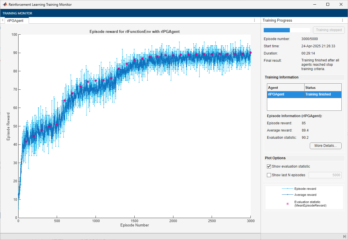
The trained agent achieves a 90.2% accuracy after 3000 episodes. With a different random seed, the initial agent network would be different, and therefore, convergence results might be different.

In general, you can achieve higher accuracy by training the agent for longer. Note that, while training times depend on many factors, for this example, training takes around half an hour. By contrast, training the network in a supervised learning setting, as shown in Create Simple Image Classification Network, takes less than one minute. This difference is mostly due to the fact that a supervised learning algorithm can fully use all the available information during training, (specifically, the information about the correct digit associated with the input image), as previously mentioned. This performance difference can increase with the number of classes to be identified. Furthermore, the cross-entropy loss function typically used for classification problems in supervised learning settings is specifically tailored to classification tasks. For these reasons, converting a supervised learning problem to a reinforcement learning problem is not recommended.

Validate Trained PG Agent

To reproduce the results of this section, set random seed and algorithm.

rng(0,"twister")

Calculate the number of images in the validation datastore.

nVal = sum(imdsValidation.countEachLabel.(2))

nVal = 
2500

Create the environment object for validation, using the validation datastore.

envVal = rlFunctionEnv(obsInfo,actInfo, ...
    @(a,x) clsfStepFcn(a,x,imdsValidation,nVal), ...
    @() clsfResetFcn(imdsValidation,nVal));

By default, the agent uses a greedy (hence deterministic) policy in simulation. To use the exploratory policy instead, set the UseExplorationPolicy agent property to true.

To simulate the trained agent, create a simulation options object and configure it to simulate for 100 steps. For more information, see rlSimulationOptions.

simOptions = rlSimulationOptions(MaxSteps=100);

Simulate the validation environment with the trained agent and display the total reward. For more information on agent simulation, see sim.

experience = sim(envVal,pgAgent,simOptions);
totalReward = sum(experience.Reward)

totalReward = 
88

This total reward value indicates that the trained agent is able to successfully classify unseen images with an accuracy of 89%.

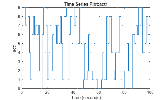
Plot the image label with time in the simulation episode.

plot(experience.Action.act1)

Display the image and the resulting action at step number 25.

sn = 25;
image(uint8(255*experience.Observation.obs1.Data(:,:,sn)))
axis("square")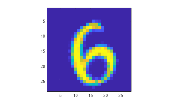

experience.Action.act1.Data(:,:,sn)

ans = 
6

The agent has classified the image correctly.

Restore the random number stream using the information stored in previousRngState.

rng(previousRngState);

This example has shown that you can convert an image classification problem into a contextual bandit problem, which you can then solve using a reinforcement learning agent. This process illustrates the main differences between the two paradigms, and why converting a supervised learning problem into a reinforcement learning problem is not recommended.

Reference

[1] Barto, Andrew G., and Thomas G. Dietterich. "Reinforcement Learning and its Relationship to Supervised Learning". 2004. https://all.cs.umass.edu/pubs/2004/barto_d_04.pdf.

[2] Slivkins, Aleksandrs. “Introduction to Multi-Armed Bandits.” arXiv, April 3, 2024. https://doi.org/10.48550/arXiv.1904.07272.