Why Solving Regression Using Reinforcement Learning is Not Recommended
This example shows how to solve a regression problem using both a supervised learning approach and a reinforcement learning approach, illustrating the differences between these methods. This example also illustrates why reinforcement learning is not the right tool to solve a supervised learning problem. For more information on the relationship between reinforcement and supervised learning, see [1].
Fix Random Number Stream for Reproducibility
The example code might involve computation of random numbers at several stages. Fixing the random number stream at the beginning of some sections in the example code preserves the random number sequence in the section every time you run it, which increases the likelihood of reproducing the results. For more information, see Results Reproducibility.
Fix the random number stream with seed 0 and random number algorithm Mersenne Twister. For more information on controlling the seed used for random number generation, see rng.
previousRngState = rng(0,"twister");The output previousRngState is a structure that contains information about the previous state of the stream. You will restore the state at the end of the example.
Function Approximation Problem
In this example, you solve a regression problem consisting in approximating the following nonlinear function:
Over the domain , , and .
To train a neural network in a supervised learning fashion you supply to the network both x and the correct f(x) over the training dataset, and the algorithm adjusts the network weights so that the network output n(x) approximates f(x). You then use unseen inputs in a validation dataset to check how well the network is able to predict the correct output.
Supervised Learning Solution
Ensure reproducibility of the section by fixing the seed used for random number generation.
rng(0,"twister")Create a training data set with 5000 data points in the function domain.
x = ([1 0 6 7]-[0 -5 -6 -2]).*rand(5e3,4) + [0 -5 -6 -2];
y = 2/30*(x(:,1).^2 + x(:,2) + x(:,3) + x(:,1).*x(:,4)) - 1/30;
Define a neural network to approximate the function. Create the network as a vector of layer objects.
layers = [
    featureInputLayer(4)
    fullyConnectedLayer(16)
    reluLayer
    fullyConnectedLayer(1)
    ];
Create a dlnetwork object and display the number of learnable parameters.
net = dlnetwork(layers);
summary(net)
   Initialized: true

   Number of learnables: 97

   Inputs:
      1   'input'   4 features
Define the training options.
opts = trainingOptions("adam",...
    InitialLearnRate=0.005,...
    LearnRateSchedule="piecewise",...
    LearnRateDropPeriod=100,...
    Plots="none",...
    Verbose=true, ...
    VerboseFrequency=500, ...
    LearnRateDropFactor=0.97,...
    GradientThreshold=1,...
    MaxEpochs=150);
Train the network using the trainnet function.
net = trainnet(x,y,net,"mse",opts); Iteration Epoch TimeElapsed LearnRate TrainingLoss
_________ _____ ___________ _________ ____________
1 1 00:00:00 0.005 4.6273
500 13 00:00:02 0.005 0.0011827
1000 26 00:00:03 0.005 0.00060518
1500 39 00:00:04 0.005 0.00043892
2000 52 00:00:04 0.005 0.00039223
2500 65 00:00:05 0.005 0.00024674
3000 77 00:00:06 0.005 0.00017821
3500 90 00:00:07 0.005 0.00012099
4000 103 00:00:07 0.00485 6.6191e-05
4500 116 00:00:08 0.00485 9.0857e-05
5000 129 00:00:09 0.00485 7.0055e-05
5500 142 00:00:09 0.00485 4.9874e-05
5850 150 00:00:10 0.00485 6.8377e-05
Training stopped: Max epochs completed
The training converges in less than 30 seconds.
Create a validation dataset with 50 points in the function domain.
x = ([1 0 6 7]-[0 -5 -6 -2]).*rand(50,4) + [0 -5 -6 -2];
y = 2/30*(x(:,1).^2 + x(:,2) + x(:,3) + x(:,1).*x(:,4)) - 1/30;
Calculate the neural network predictions using the predict function.
z = predict(net,x);
Plot the true function value against the approximation, displaying the norm of the difference.
plot(1:50,[y z]); legend("y","z")
xlabel("time"); ylabel("y & z");
title(['Norm(y-z) = ' num2str(norm(y-z))]);
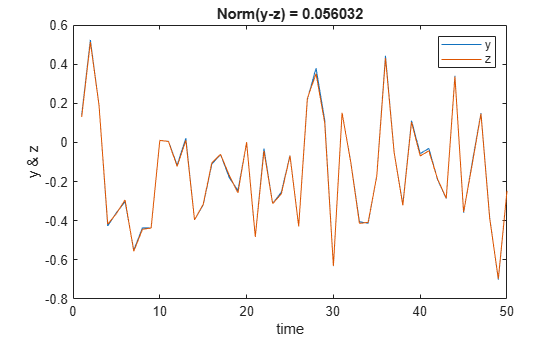
The trained network successfully approximates the function.
Reinforcement Learning Solution: Contextual Bandit Framework
You can express this function approximation problem as a reinforcement learning problem. During reinforcement learning training, your environment supplies to an agent both x (the observation) and a scalar reward that is higher the closer the agent output a(x) (the action) approximates f(x). Note that the reward only captures the information of how close a(x) is to f(x) but the full knowledge of f(x) is not available to the agent. By contrast, this information is fully used in the supervised learning setting, (which is why training is generally much faster for supervised learning).
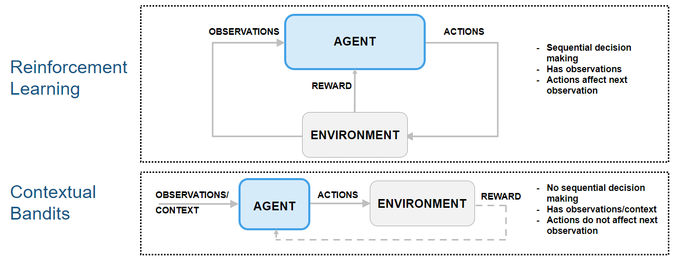
Because the next observation is independent of the action, this type of reinforcement learning problem can be classified as a "contextual bandit" problem. In contextual bandits problems, the environment has no state dynamics, so the reward is only influenced by the current observation and action.
The following figure shows how contextual bandit problems are special cases of reinforcement learning problems.
For an example that shows how to use an agent to solve a contextual bandit problem, see Train Reinforcement Learning Agent for Simple Contextual Bandit Problem. For an example discussing classification as a contextual bandit problems, see Why Solving Classification Using Reinforcement Learning Is Not Recommended. For a comprehensive introduction to bandit problems, see [2].
Create Custom Continuous-Action-Space Environment Object
Create the environment specifications. The observation (state) is the current value of x, and the action is the estimated value of the function, a(x).
obsInfo = rlNumericSpec([4 1], ...
    LowerLimit=[0 -5 -6 -2]', ...
    UpperLimit=[1 0 6 7]');
actInfo = rlNumericSpec([1 1], ...
    LowerLimit=-1, ...
    UpperLimit=1);
At the beginning of each training or simulation episode, a reset function resets the environment to an initial state and returns both the initial state (needed for the next environment step) and the resulting initial observation value (for the agent to see).
Display the custom reset function, which is provided in the file rgsnfResetFcn.m.
type("rgsnResetFcn.m")function [obs0,x0] = rgsnResetFcn() % Reset function to set environment in random initial state. % Return initial observation and state. x0 = ([1 0 6 7]-[0 -5 -6 -2])'.*rand(4,1) + [0 -5 -6 -2]'; obs0 = x0; end
This function takes no input argument, calculates a random initial point in the domain, and returns it both as initial observation and state.
A step function is called by train (or sim) at each step of the training (or simulation) episode to advance the environment to the next step.
Display the custom step function, which is provided in the file rgsnStepFcn.m.
type("rgsnStepFcn.m")function [nextObs,r,isdn,xp] = rgsnStepFcn(a,x)
% Custom step function to advance custom environment by one step
% Initialize is-done.
isdn = 0;
% Make sure action is finite; otherwise, terminate.
if ~allfinite(a)
isdn = 1;
a(~isfinite(a)) = rand;
end
% Calculate true function value.
f_star = 2/30*(x(1)^2 + x(2) + x(3) + x(1)*x(4)) - 1/30;
% Calculate reward (reward for a).
r = 0.1-norm(a-f_star);
% Make sure reward value is finite; otherwise, terminate.
if ~allfinite(r)
isdn = 1;
r(~isfinite(r)) = -1e20;
end
% Calculate next observation and state.
% Calculate random action-independent feasible point.
p = ([1 0 6 7]-[0 -5 -6 -2])'.*rand(4,1) + [0 -5 -6 -2]';
% Move current state toward p, ans set next obs = next state.
xp = x + 0.2*(p-x);
nextObs = xp;
end
This function takes the action from the agent and the current environment state as input arguments. It then uses the current state to calculate the true function value, f_star, which is in turn used to calculate the reward that the agent receives for the action a. The reward decreases proportionally to the Euclidean distance between the action and the true function value. If the distance is less than 0.1, the reward is positive.
The step function then calculates the next state by moving the current state toward a random point in the domain, setting the next observation to the next state.
If the received action or calculated reward is non-finite, the is-done flag is set to one, which causes the episode to terminate.
Create the custom function environment object, passing the observation and action specifications and the handles of the custom step and reset functions to the rlFunctionEnv function.
env = rlFunctionEnv(obsInfo,actInfo, @rgsnStepFcn, @rgsnResetFcn);
For a more detailed example on custom step and reset functions, see Create Custom Environment Using Step and Reset Functions.
Create DDPG Agent and Specify Agent Options
The actor and critic networks are initialized randomly. Specify random seed and algorithm for reproducibility.
rng(0,"twister")Create a default rlDDPGAgent object using the environment specification objects.
ddpgAgent = rlDDPGAgent(obsInfo,actInfo);
Set a lower learning rate and gradient thresholds to avoid instability.
ddpgAgent.AgentOptions.CriticOptimizerOptions.LearnRate = 1e-3;
ddpgAgent.AgentOptions.ActorOptimizerOptions.LearnRate = 1e-3;
ddpgAgent.AgentOptions.CriticOptimizerOptions.GradientThreshold = 1;
ddpgAgent.AgentOptions.ActorOptimizerOptions.GradientThreshold = 1;
Because future reward is independent on the action, set a discount factor of zero.
ddpgAgent.AgentOptions.DiscountFactor = 0;
Configure Training Options
Create an evaluator object to evaluate the agent five times without exploration every 100 episodes.
evl = rlEvaluator(NumEpisodes=5,EvaluationFrequency=100);
Create a training options object. For more information, see rlTrainingOptions.
trainOpts = rlTrainingOptions;
Specify training options. For this example:
Set the maximum number of steps per episode to
500(note that the environment has no terminal state).Stop the training when the average reward collected over the evaluation episodes reaches 48 (in this example, the maximum reward over an episode is 0.1*500 = 50).
In any case, stop after 1000 episodes.
trainOpts.MaxEpisodes = 1000;
trainOpts.MaxStepsPerEpisode = 500;
trainOpts.StopTrainingCriteria = "EvaluationStatistic";
trainOpts.StopTrainingValue = 48;
Alternatively, because the next state is independent of the action, you can set the maximum number of steps per episode to 1 (and consequently allow for a larger number of episodes). Adopting this view, each episode is a stand-alone event in which the agent associates a single observation to a single action, that is, each episode represents an instance of a bandit problem with a different context (a different input value). You must use this approach if your environment does not allow multiple steps per episode.
However, if you use this alternative approach to train agents like PG agents, which calculate network gradients at the end of the episode and use only the steps available in the episode, then the network gradients are calculated using only a single observation and reward. This can lead to inefficient or unstable learning.
For an example using this alternative approach, see Train Reinforcement Learning Agent for Simple Contextual Bandit Problem.
Train the DDPG Agent
To reproduce the results of this section, set random seed and algorithm.
rng(0,"twister")To train the agent, pass the agent, the environment, the training options, and the evaluator objects to train. Training is a computationally intensive process that takes several minutes to complete. To save time while running this example, load a pretrained agent by setting doTraining to false. To train the agent yourself, set doTraining to true.
doTraining =false; if doTraining % Train the agent. Save the final agent and training results. pgTrainingRes = train(ddpgAgent,env,trainOpts,Evaluator=evl); % Uncomment to save the trained agent and results. % save("rgsnDDPGAgent.mat","ddpgAgent","pgTrainingRes") else % Load the pretrained agent and results for the example. load("rgsnDDPGAgent.mat","ddpgAgent","pgTrainingRes") end
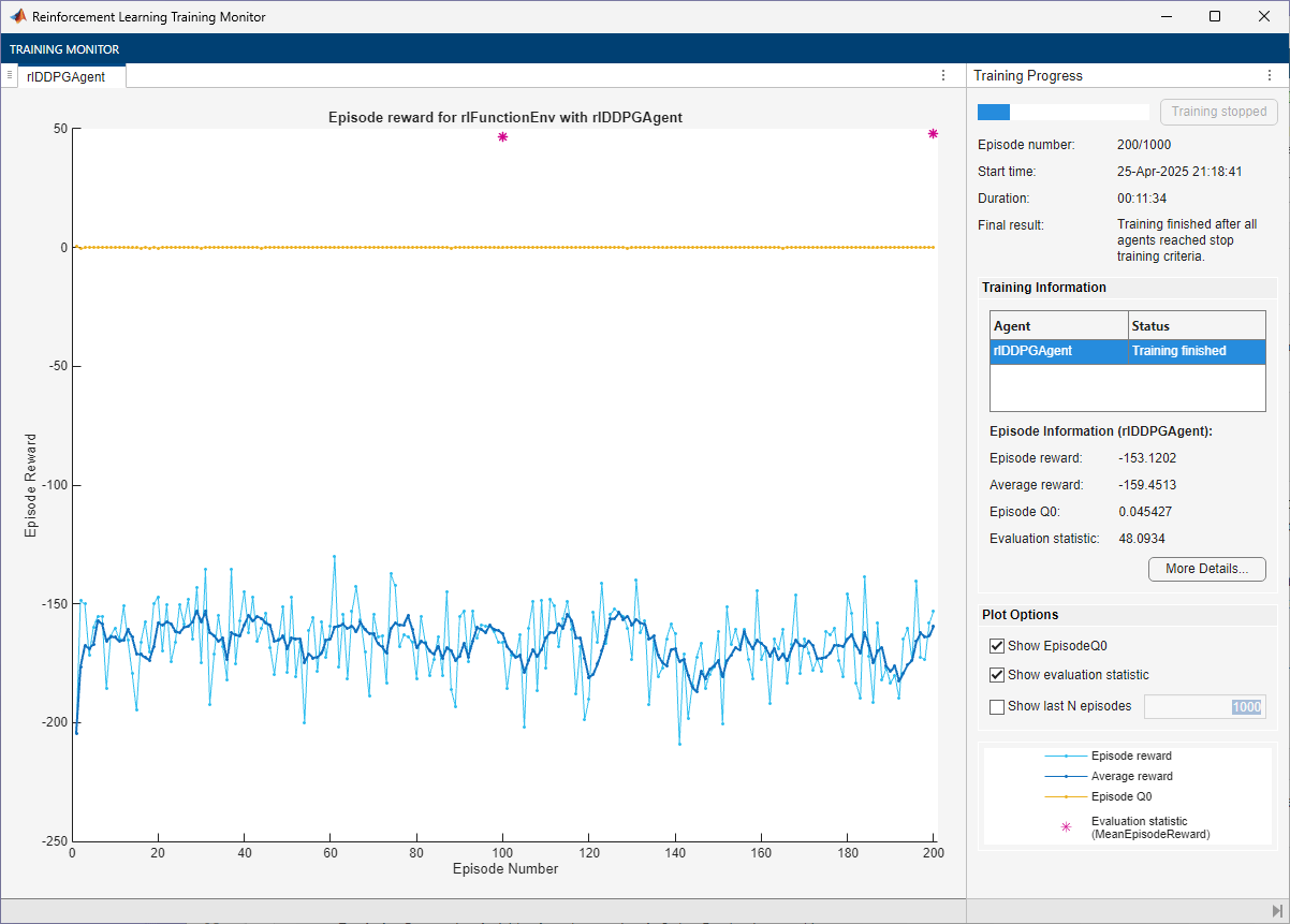
The trained agent achieves a reward of 48 after 200 episodes. With a different random seed, the initial agent networks would be different, so convergence results might be different.
In general, you might achieve higher accuracy by training the agent for longer. Note that, while training times depend on many factors, for this example, training takes more than ten minutes. By contrast, training the network in a supervised learning setting, as shown in the related previous section, takes less than 30 seconds. This difference is mostly due to the fact that a supervised learning algorithm can fully use all the available information during training (specifically, the information about the correct value of the function output associated with the observation), as previously mentioned. This performance difference can increase with the number dimensions of the function output. For these reasons, converting a supervised learning problem to a reinforcement learning problem is not recommended.
Validate Trained DDPG Agent
To reproduce the results of this section, set random seed and algorithm.
rng(1,"twister")By default, the agent uses a greedy (hence deterministic) policy in simulation. To use the exploratory policy instead, set the UseExplorationPolicy agent property to true.
To simulate the trained agent, create a simulation options object and configure it to simulate for 50 steps. For more information, see rlSimulationOptions.
simOptions = rlSimulationOptions(MaxSteps=50);
Simulate the environment with the trained agent and display the total reward. For more information on agent simulation, see sim.
experience = sim(env,ddpgAgent,simOptions);
totalReward = sum(experience.Reward)
totalReward =
4.6846
This total reward value indicates that the trained agent is able to approximate the function with adequate accuracy.
Plot the true function value against the approximation, displaying the norm of the difference.
x = zeros(50,4);
for i=1:4
    x(:,i) = squeeze(experience.Observation.obs1.Data(i,1,1:end-1));
end
y = 2/30*(x(:,1).^2 + x(:,2) + x(:,3) + x(:,1).*x(:,4)) - 1/30;
t = experience.Action.act1.Time;
a = squeeze(experience.Action.act1.Data(1,1,:));
plot(t,[y a]); legend("y","a")
xlabel("time"); ylabel("y & a");
title(['Norm(y-a) = ' num2str(norm(y-a))]);
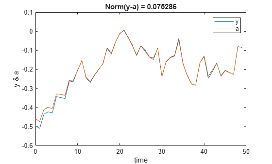
The figure confirms that the agent is able to approximate the function at least in this region of the observation space.
Restore the random number stream using the information stored in previousRngState.
rng(previousRngState);
This example has shown that you can convert a function approximation problem into a contextual bandit problem, which you can then solve using a reinforcement learning agent. This process illustrates the main differences between the two paradigms, and why converting a supervised learning problem into a reinforcement learning problem is not recommended.
Reference
[1] Barto, Andrew G., and Thomas G. Dietterich. "Reinforcement Learning and its Relationship to Supervised Learning". 2004. https://all.cs.umass.edu/pubs/2004/barto_d_04.pdf.
[2] Slivkins, Aleksandrs. “Introduction to Multi-Armed Bandits.” arXiv, April 3, 2024. https://doi.org/10.48550/arXiv.1904.07272.