fplot
Plot symbolic expression or function
Syntax
Description
fplot(
plots f,[xmin xmax])f over the interval [xmin
xmax].
fplot( plots xt,yt,[tmin
tmax])xt = x(t) and yt =
y(t) over the specified range [tmin
tmax].
fplot(___,
specifies line properties using one or more Name=Value)Name=Value
arguments. Use this option with any of the input argument combinations in the
previous syntaxes. Name=Value settings apply to all the lines
plotted. To set options for individual lines, use the objects returned by
fplot.
fplot( plots into
the axes specified by ax,___)ax instead of the current axes
gca.
fp = fplot(___)
Examples
Plot tan(x) over the default range [-5 5]. fplot shows poles by default. For details, see the ShowPoles argument in Name-Value Arguments.
syms x
fplot(tan(x))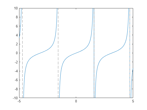
Plot the symbolic function f(x) = cos(x) over the default range [-5 5].
syms f(x)
f(x) = cos(x);
fplot(f)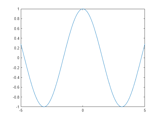
Plot the parametric curve x = cos(3*t) and y = sin(2*t).
syms t
x = cos(3*t);
y = sin(2*t);
fplot(x,y)
Plot sin(x) over [-pi/2 pi/2] by specifying the plotting interval as the second input to fplot.
syms x
fplot(sin(x),[-pi/2 pi/2])
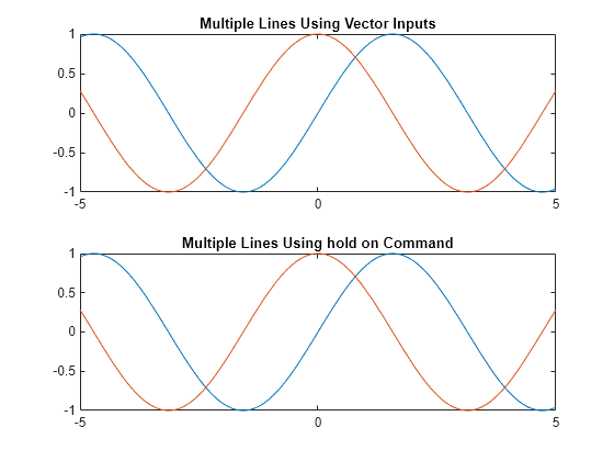
You can plot multiple lines either by passing the inputs as a vector or by using hold on to successively plot on the same figure. If you specify LineSpec and Name-Value arguments, they apply to all lines. To set options for individual plots, use the function handles returned by fplot.
Divide a figure into two subplots using subplot. On the first subplot, plot sin(x) and cos(x) using vector input. On the second subplot, plot sin(x) and cos(x) using hold on.
syms x
tiledlayout(2,1)
nexttile
fplot([sin(x) cos(x)])
title("Multiple Lines Using Vector Inputs")

nexttile
fplot(sin(x))
hold on
fplot(cos(x))
title("Multiple Lines Using hold on Command")

hold off
Plot three sine curves with a phase shift between each line. For the first line, use a linewidth of 2. For the second, specify a dashed red line style with circle markers. For the third, specify a cyan, dash-dot line style with asterisk markers. Display the legend.
syms x
fplot(sin(x+pi/5),Linewidth=2)
hold on
fplot(sin(x-pi/5),"--or")
fplot(sin(x),"-.*c")
legend(Location="best")
hold off

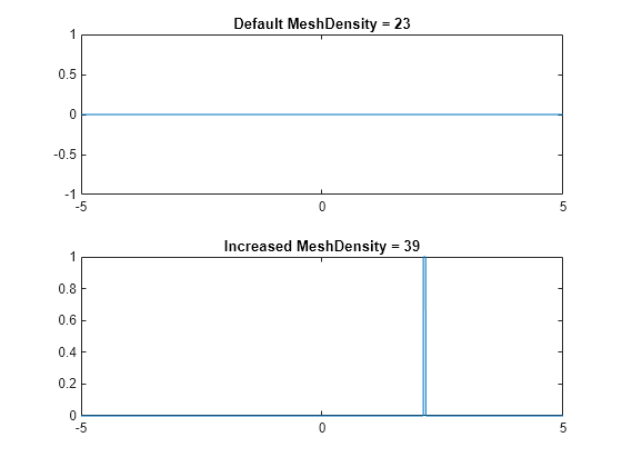
Control the resolution of a plot by using the MeshDensity option. Increasing MeshDensity can make smoother, more accurate plots, while decreasing it can increase plotting speed.
Divide a figure into two by using subplot. In the first subplot, plot a step function from x = 2.1 to x = 2.15. The plot's resolution is too low to detect the step function. Fix this issue by increasing MeshDensity to 39 in the second subplot. The plot now detects the step function and shows that by increasing MeshDensity you increased the plot's resolution.
syms x
stepFn = rectangularPulse(2.1, 2.15, x);

subplot(2,1,1)
fplot(stepFn);
title("Default MeshDensity = 23")

subplot(2,1,2)
fplot(stepFn,MeshDensity=39);
title("Increased MeshDensity = 39")
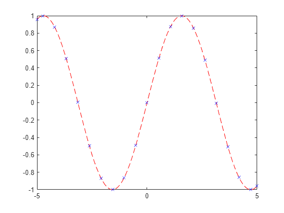
Plot sin(x). Specify an output to make fplot return the plot object.
syms x
h = fplot(sin(x))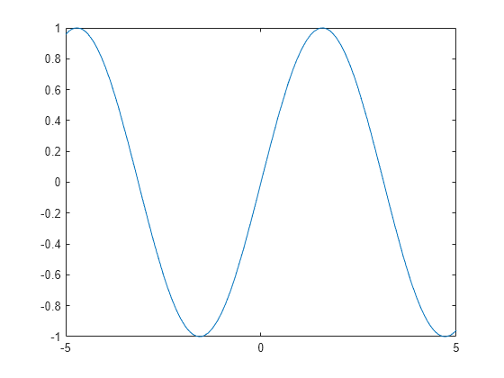
h =
  FunctionLine with properties:

     Function: sin(x)
        Color: [0.0660 0.4430 0.7450]
    LineStyle: '-'
    LineWidth: 0.5000

  Show all properties
Change the default blue line to a dashed red line by using dot notation to set properties. Similarly, add "x" marker and set the marker color to blue.
h.LineStyle = "--";
h.Color = "r";
h.Marker = "x";
h.MarkerEdgeColor = "b";
Plot sin(x) over the interval [-2*pi 2*pi]. Add a title and axis labels. Create the -axis ticks by spanning the -axis limits at intervals of pi/2. Display these ticks by using the XTick property. Create -axis labels by using arrayfun to apply texlabel to S. Display these labels by using the XTickLabel property.
To use LaTeX in plots, see latex.
syms x
fplot(sin(x),[-2*pi 2*pi])
grid on
title("sin(x) from -2\pi to 2\pi")
xlabel("x")
ylabel("y")

ax = gca;
S = sym(ax.XLim(1):pi/2:ax.XLim(2));
ax.XTick = double(S);
ax.XTickLabel = arrayfun(@texlabel,S,UniformOutput=false);

When you zoom into a plot, fplot reevaluates the plot automatically. The reevaluation when zooming reveals more details at smaller scales.
Plot the curve  for
for  and
and  . Zoom into the plot using
 zoom and redraw the plot using drawnow. Because of reevaluation on zoom, fplot reveals more details. Repeat the zoom 6 times to view smaller-scale details.
syms x
fplot(x^3*sin(1/x));
axis([-2 2 -0.02 0.02]);
for i=1:6
    zoom(1.7)
    pause(0.5)
end

Create an animation of a parametric curve where one of the parameters changes with time. The  - and
- and  -coordinates of the parametric curve are given by


By varying the variable  from 0.1 to 3, animate the parametric curve.
Create two symbolic variables k and t. Use the variable k to parameterize the curve within the range [-5 5] and use the variable t to animate the curve as the time proceeds from 0.1 to 3. Create a stop-motion animation object of the time snapshots by using fanimator. Set the -axis and -axis to be equal length.
syms k t
fanimator(@fplot,k*t*sin(k*t),k*t*cos(k*t),[-5 5],AnimationRange = [0.1 3])
axis equal

Play the animation by using playAnimation.
playAnimation

You can also save the animation as a GIF file by using writeAnimation.
writeAnimation("parametricCurve.gif")

Input Arguments
Expression or function to plot, specified as a symbolic expression or function.
Plotting interval for x-coordinates, specified as a
vector of two numbers. The default range is [-5 5].
However, if fplot detects a finite number of
discontinuities in f, then fplot
expands the range to show them.
Parametric input for x-coordinates, specified as a
symbolic expression or function. fplot uses
symvar to find the parameter.
Parametric input for y-axis, specified as a symbolic
expression or function. fplot uses
symvar to find the parameter.
Range of values of parameter t, specified as a vector
of two numbers. The default range is [-5 5].
Axes object. If you do not specify an axes object, then
fplot uses the current axes
gca.
Line style, marker, and color, specified as a string scalar or character vector containing symbols. The symbols can appear in any order. You do not need to specify all three characteristics (line style, marker, and color). For example, if you omit the line style and specify the marker, then the plot shows only the marker and no line.
Example: "--or" is a red dashed line with circle markers.
| Line Style | Description | Resulting Line |
|---|---|---|
"-" | Solid line |
|
"--" | Dashed line |
|
":" | Dotted line |
|
"-." | Dash-dotted line |
|
| Marker | Description | Resulting Marker |
|---|---|---|
"o" | Circle |
|
"+" | Plus sign |
|
"*" | Asterisk |
|
"." | Point |
|
"x" | Cross |
|
"_" | Horizontal line |
|
"|" | Vertical line |
|
"square" | Square |
|
"diamond" | Diamond |
|
"^" | Upward-pointing triangle |
|
"v" | Downward-pointing triangle |
|
">" | Right-pointing triangle |
|
"<" | Left-pointing triangle |
|
"pentagram" | Pentagram |
|
"hexagram" | Hexagram |
|
| Color Name | Short Name | RGB Triplet | Appearance |
|---|---|---|---|
"red" | "r" | [1 0 0] |
|
"green" | "g" | [0 1 0] |
|
"blue" | "b" | [0 0 1] |
|
"cyan"
| "c" | [0 1 1] |
|
"magenta" | "m" | [1 0 1] |
|
"yellow" | "y" | [1 1 0] |
|
"black" | "k" | [0 0 0] |
|
"white" | "w" | [1 1 1] |
|
Name-Value Arguments
Specify optional pairs of arguments as
Name1=Value1,...,NameN=ValueN, where Name is
the argument name and Value is the corresponding value.
Name-value arguments must appear after other arguments, but the order of the
pairs does not matter.
Before R2021a, use commas to separate each name and value, and enclose
Name in quotes.
Example: Marker="o",MarkerFaceColor="red"
The function line properties listed here are only a subset. For a complete list, see FunctionLine Properties.
Display asymptotes at poles, specified as "on" or
"off", or as numeric or logical
1 (true) or
0 (false). A value of
"on" is equivalent to true, and
"off" is equivalent to false.
Thus, you can use the value of this property as a logical value. The
value is stored as an on/off logical value of type matlab.lang.OnOffSwitchState.
The asymptotes display as gray, dashed vertical lines.
fplot displays asymptotes only with the
fplot(f) syntax or variants, and not with the
fplot(xt,yt) syntax.
Alternatively, you can specify some common colors by name. This table lists the named color options, the equivalent RGB triplets, and the hexadecimal color codes.
| Color Name | Short Name | RGB Triplet | Hexadecimal Color Code | Appearance |
|---|---|---|---|---|
"red" | "r" | [1 0 0] | "#FF0000" |
|
"green" | "g" | [0 1 0] | "#00FF00" |
|
"blue" | "b" | [0 0 1] | "#0000FF" |
|
"cyan"
| "c" | [0 1 1] | "#00FFFF" |
|
"magenta" | "m" | [1 0 1] | "#FF00FF" |
|
"yellow" | "y" | [1 1 0] | "#FFFF00" |
|
"black" | "k" | [0 0 0] | "#000000" |
|
"white" | "w" | [1 1 1] | "#FFFFFF" |
|
This table lists the default color palettes for plots in the light and dark themes.
| Palette | Palette Colors |
|---|---|
Before R2025a: Most plots use these colors by default. |
|
|
|
You can get the RGB triplets and hexadecimal color codes for these palettes using the orderedcolors and rgb2hex functions. For example, get the RGB triplets for the "gem" palette and convert them to hexadecimal color codes.
RGB = orderedcolors("gem");
H = rgb2hex(RGB);
Before R2023b: Get the RGB triplets using RGB =
get(groot,"FactoryAxesColorOrder").
Before R2024a: Get the hexadecimal color codes using H =
compose("#%02X%02X%02X",round(RGB*255)).
Example: "blue"
Example: [0
0 1]
Example: "#0000FF"
Line style, specified as one of the options listed in this table.
| Line Style | Description | Resulting Line |
|---|---|---|
"-" | Solid line |
|
"--" | Dashed line |
|
":" | Dotted line |
|
"-." | Dash-dotted line |
|
"none" | No line | No line |
Marker symbol, specified as one of the values listed in this table. By default, the object does not display markers. Specifying a marker symbol adds markers at each data point or vertex.
| Marker | Description | Resulting Marker |
|---|---|---|
"o" | Circle |
|
"+" | Plus sign |
|
"*" | Asterisk |
|
"." | Point |
|
"x" | Cross |
|
"_" | Horizontal line |
|
"|" | Vertical line |
|
"square" | Square |
|
"diamond" | Diamond |
|
"^" | Upward-pointing triangle |
|
"v" | Downward-pointing triangle |
|
">" | Right-pointing triangle |
|
"<" | Left-pointing triangle |
|
"pentagram" | Pentagram |
|
"hexagram" | Hexagram |
|
"none" | No markers | Not applicable |
Alternatively, you can specify some common colors by name. This table lists the named color options, the equivalent RGB triplets, and the hexadecimal color codes.
| Color Name | Short Name | RGB Triplet | Hexadecimal Color Code | Appearance |
|---|---|---|---|---|
"red" | "r" | [1 0 0] | "#FF0000" |
|
"green" | "g" | [0 1 0] | "#00FF00" |
|
"blue" | "b" | [0 0 1] | "#0000FF" |
|
"cyan"
| "c" | [0 1 1] | "#00FFFF" |
|
"magenta" | "m" | [1 0 1] | "#FF00FF" |
|
"yellow" | "y" | [1 1 0] | "#FFFF00" |
|
"black" | "k" | [0 0 0] | "#000000" |
|
"white" | "w" | [1 1 1] | "#FFFFFF" |
|
"none" | Not applicable | Not applicable | Not applicable | No color |
This table lists the default color palettes for plots in the light and dark themes.
| Palette | Palette Colors |
|---|---|
Before R2025a: Most plots use these colors by default. |
|
|
|
You can get the RGB triplets and hexadecimal color codes for these palettes using the orderedcolors and rgb2hex functions. For example, get the RGB triplets for the "gem" palette and convert them to hexadecimal color codes.
RGB = orderedcolors("gem");
H = rgb2hex(RGB);
Before R2023b: Get the RGB triplets using RGB =
get(groot,"FactoryAxesColorOrder").
Before R2024a: Get the hexadecimal color codes using H =
compose("#%02X%02X%02X",round(RGB*255)).
Example: [0.3 0.2 0.1]
Example: "green"
Example: "#D2F9A7"
Output Arguments
Tips
If
fplotdetects a finite number of discontinuities inf, thenfplotexpands the range to show them.If
fplotis used with a function handle to a named or anonymous function (that is not a symbolic expression or function), then the MATLAB®fplotfunction is called. In this case, the function handle must accept a vector input argument and return a vector output argument of the same size. Use array operators instead of matrix operators for the best performance. For example, use.*(times) instead of*(mtimes) in the codefplot(@(x) x.*sin(2*pi*x)).
Version History
Introduced in R2016a