fsurf
Plot 3-D surface
Syntax
Description
fsurf( creates a
surface plot of the symbolic expression f)f(x,y) over
the default interval [-5 5] for x and y.
fsurf(
plots f,[xmin xmax
ymin ymax])f(x,y) over the interval [xmin xmax]
for x and [ymin ymax] for
y. The fsurf function uses
symvar to order the variables and assign intervals.
fsurf( plots
the parametric surface funx,funy,funz)x = x(u,v), y =
y(u,v), z = z(u,v) over the interval [-5
5] for u and v.
fsurf( plots the parametric surface funx,funy,funz,[uvmin
uvmax])x
= x(u,v), y = y(u,v), z = z(u,v) over
the interval [uvmin uvmax] for u and v.
fsurf(
plots the parametric surface funx,funy,funz,[umin
umax vmin vmax])x = x(u,v), y =
y(u,v), z = z(u,v) over the interval
[umin umax] for u and [vmin
vmax] for v. The fsurf function uses
symvar to order the parametric variables and assign intervals.
fsurf(___, uses
LineSpec)LineSpec to set the line style, marker symbol, and face
color. Use this option after any of the previous input argument
combinations.
fsurf(___, specifies line
properties using one or more Name,Value)Name,Value pair arguments. Use
this option after any of the input argument combinations in the previous
syntaxes.
fsurf( plots
into the axes with the object ax,___)ax instead of the
current axes object gca.
fs = fsurf(___)
Examples
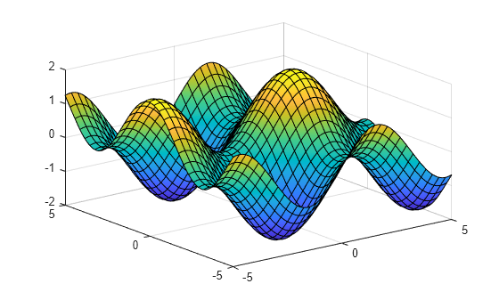
Plot the input over the default range and .
syms x y
fsurf(sin(x)+cos(y))
Plot the real part of over the default range and .
syms f(x,y)
f(x,y) = real(atan(x + i*y));
fsurf(f)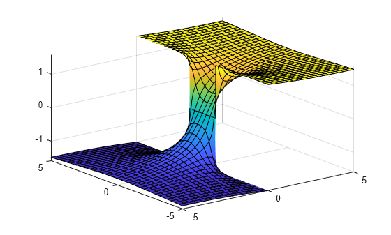
Plot over and by specifying the plotting interval as the second argument of fsurf.
syms x y
f = sin(x) + cos(y);
fsurf(f, [-pi pi -5 5])

Plot the parameterized surface
for and .
Improve the plot's appearance by using camlight.
syms s t
r = 2 + sin(7*s + 5*t);
x = r*cos(s)*sin(t);
y = r*sin(s)*sin(t);
z = r*cos(t);
fsurf(x, y, z, [0 2*pi 0 pi])
camlight
view(46,52)

Plot the piecewise expression of the Klein bottle
for and .
Show that the Klein bottle has only a one-sided surface.
syms u v;
r = @(u) 4 - 2*cos(u);
x = piecewise(u <= pi, -4*cos(u)*(1+sin(u)) - r(u)*cos(u)*cos(v),...
    u > pi, -4*cos(u)*(1+sin(u)) + r(u)*cos(v));
y = r(u)*sin(v);
z = piecewise(u <= pi, -14*sin(u) - r(u)*sin(u)*cos(v),...
    u > pi, -14*sin(u));
h = fsurf(x,y,z, [0 2*pi 0 2*pi]);

For and from to , plot the 3-D surface . Add a title and axis labels.
Create the x-axis ticks by spanning the x-axis limits at intervals of pi/2. Convert the axis limits to precise multiples of pi/2 by using round and get the symbolic tick values in S. Display these ticks by using the XTick property. Create x-axis labels by using arrayfun to apply texlabel to S. Display these labels by using the XTickLabel property. Repeat these steps for the y-axis.
To use LaTeX in plots, see latex.
syms x y
fsurf(y.*sin(x)-x.*cos(y), [-2*pi 2*pi])
title('ysin(x) - xcos(y) for x and y in [-2\pi,2\pi]')
xlabel('x')
ylabel('y')
zlabel('z')

ax = gca;
S = sym(ax.XLim(1):pi/2:ax.XLim(2));
S = sym(round(vpa(S/pi*2))*pi/2);
ax.XTick = double(S);
ax.XTickLabel = arrayfun(@texlabel,S,'UniformOutput',false);

S = sym(ax.YLim(1):pi/2:ax.YLim(2));
S = sym(round(vpa(S/pi*2))*pi/2);
ax.YTick = double(S);
ax.YTickLabel = arrayfun(@texlabel,S,'UniformOutput',false);
![Figure contains an axes object. The axes object with title ysin(x) - xcos(y) for x and y in [- 2 pi , 2 pi ], xlabel x, ylabel y contains an object of type functionsurface.](../examples/symbolic/win64/AddTitleAndAxisLabelsAndFormatTicksExample_01.png)
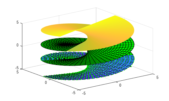
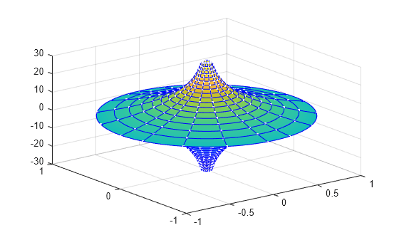
Plot the parametric surface , , with different line styles for different values of . For , use a dashed line with green dot markers. For , use a LineWidth of 1 and a green face color. For , turn off the lines by setting EdgeColor to none.
syms s t
fsurf(s*sin(t),-s*cos(t),t,[-5 5 -5 -2],'--.','MarkerEdgeColor','g')
hold on
fsurf(s*sin(t),-s*cos(t),t,[-5 5 -2 2],'LineWidth',1,'FaceColor','g')
fsurf(s*sin(t),-s*cos(t),t,[-5 5 2 5],'EdgeColor','none')
Plot the parametric surface
Specify an output to make fcontour return the plot object.
syms u v
x = exp(-abs(u)/10).*sin(5*abs(v));
y = exp(-abs(u)/10).*cos(5*abs(v));
z = u;
fs = fsurf(x,y,z)
fs =
  ParameterizedFunctionSurface with properties:

    XFunction: exp(-abs(u)/10)*sin(5*abs(v))
    YFunction: exp(-abs(u)/10)*cos(5*abs(v))
    ZFunction: u
    EdgeColor: [0 0 0]
    LineStyle: '-'
    FaceColor: 'interp'

  Show all properties
Change the range of u to [-30 30] by using the URange property of fs. Set the line color to blue by using the EdgeColor property and specify white, dot markers by using the Marker and MarkerEdgeColor properties.
fs.URange = [-30 30];
fs.EdgeColor = 'b';
fs.Marker = '.';
fs.MarkerEdgeColor = 'w';
Plot multiple surfaces using vector input to fsurf. Alternatively, use hold on to plot successively on the same figure. When displaying multiple surfaces on the same figure, transparency is useful. Adjust the transparency of surface plots by using the FaceAlpha property. FaceAlpha varies from 0 to 1, where 0 is full transparency and 1 is no transparency.
Plot the planes and using vector input to fsurf. Show both planes by making them half transparent using FaceAlpha.
syms x y
h = fsurf([x+y x-y]);
h(1).FaceAlpha = 0.5;
h(2).FaceAlpha = 0.5;
title('Planes (x+y) and (x-y) at half transparency')

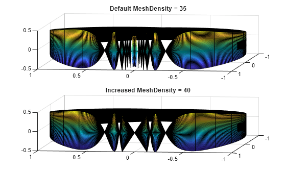
Control the resolution of a surface plot using the 'MeshDensity' option. Increasing 'MeshDensity' can make smoother, more accurate plots while decreasing it can increase plotting speed.
Divide a figure into two using subplot. In the first subplot, plot the parametric surface , , and . The surface has a large gap. Fix this issue by increasing the 'MeshDensity' to 40 in the second subplot. fsurf fills the gap showing that by increasing 'MeshDensity' you increased the plot's resolution.
syms s t

subplot(2,1,1)
fsurf(sin(s), cos(s), t/10.*sin(1./s))
view(-172,25)
title('Default MeshDensity = 35')

subplot(2,1,2)
fsurf(sin(s), cos(s), t/10.*sin(1./s),'MeshDensity',40)
view(-172,25)
title('Increased MeshDensity = 40')
Show contours for the surface plot of the expression f by setting the 'ShowContours' option to 'on'.
syms x y
f = 3*(1-x)^2*exp(-(x^2)-(y+1)^2)...
- 10*(x/5 - x^3 - y^5)*exp(-x^2-y^2)...
- 1/3*exp(-(x+1)^2 - y^2);
fsurf(f,[-3 3],'ShowContours','on')

Create an animation of surface plots by changing the displayed expression using the Function, XFunction, YFunction, and ZFunction properties, and then use drawnow to update the plot. To export to GIF, see imwrite.
By varying the variable  from 1 to 3, animate the parametric surface


for  and
and  . Increase plotting speed by reducing
 MeshDensity to 9.
syms s t
h = fsurf(t.*sin(s), cos(s), sin(1./s), [-0.1 0.1 0 1]);
h.MeshDensity = 9;
for i=1:0.1:3
    h.ZFunction = sin(i./s);
    drawnow
end

Create a symbolic expression f for the function
Plot the expression f as a surface. Improve the appearance of the surface plot by using the properties of the handle returned by fsurf, the lighting properties, and the colormap.
Create a light by using camlight. Increase brightness by using brighten. Remove the lines by setting EdgeColor to 'none'. Increase the ambient light using AmbientStrength. For details, see Lighting, Transparency, and Shading. Turn the axes box on. For the title, convert f to LaTeX using latex. Finally, to improve the appearance of the axes ticks, axes labels, and title, set 'Interpreter' to 'latex'.
syms x y
f = 3*(1-x)^2*exp(-(x^2)-(y+1)^2)...
   - 10*(x/5 - x^3 - y^5)*exp(-x^2-y^2)...
   - 1/3*exp(-(x+1)^2 - y^2);
h = fsurf(f,[-3 3]);

camlight(110,70)
brighten(0.6)
h.EdgeColor = 'none';
h.AmbientStrength = 0.4;

a = gca;
a.TickLabelInterpreter = 'latex';
a.Box = 'on';
a.BoxStyle = 'full';

xlabel('$x$','Interpreter','latex')
ylabel('$y$','Interpreter','latex')
zlabel('$z$','Interpreter','latex')
title_latex = ['$' latex(f) '$'];
title(title_latex,'Interpreter','latex')

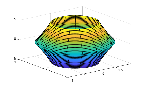
Plot a cylindrical shell bounded below by the plane and above by the plane .
syms r t u
fsurf(cos(t),sin(t),u*(cos(t)+2),[0 2*pi 0 1])
hold on;
Add a surface plot of the plane .
fsurf(r*cos(t),r*sin(t),r*cos(t)+2,[0 1 0 2*pi])

Apply rotation and translation to the surface plot of a torus.
A torus can be defined parametrically by
where
is the polar angle and is the azimuthal angle
is the radius of the tube
is the distance from the center of the tube to the center of the torus
Define the values for and as 1 and 5, respectively. Plot the torus using fsurf.
syms theta phi
a = 1;
R = 4;
x = (R + a*cos(theta))*cos(phi);
y = (R + a*cos(theta))*sin(phi);
z = a*sin(theta);
fsurf(x,y,z,[0 2*pi 0 2*pi])
hold on
Apply rotation to the torus around the -axis. Define the rotation matrix. Rotate the torus by 90 degrees or radians.
alpha = pi/2;
Rx = [1 0 0;
      0 cos(alpha) -sin(alpha);
      0 sin(alpha) cos(alpha)];
r = [x; y; z];
r_90 = Rx*r;
Shift the center of the torus by 5 along the -axis. Add a second plot of the rotated and translated torus to the existing graph.
fsurf(r_90(1)+5,r_90(2),r_90(3))
axis([-5 10 -5 10 -5 5])
hold off
Input Arguments
Expression or function to be plotted, specified as a symbolic expression or function.
Plotting interval for x- and y-axes, specified as a vector of
two numbers. The default is [-5 5].
Plotting interval for x- and y-axes, specified as a vector of
four numbers. The default is [-5 5 -5 5].
Parametric functions of u and v,
specified as a symbolic expression or function.
Plotting interval for u and v axes,
specified as a vector of two numbers. The default is [-5
5].
Plotting interval for u and v,
specified as a vector of four numbers. The default is [-5
5 -5 5].
Axes object. If you do not specify an axes object, then fsurf uses
the current axes.
Line style, marker, and color, specified as a string scalar or character vector containing symbols. The symbols can appear in any order. You do not need to specify all three characteristics (line style, marker, and color). For example, if you omit the line style and specify the marker, then the plot shows only the marker and no line.
Example: "--or" is a red dashed line with circle markers.
| Line Style | Description | Resulting Line |
|---|---|---|
"-" | Solid line |
|
"--" | Dashed line |
|
":" | Dotted line |
|
"-." | Dash-dotted line |
|
| Marker | Description | Resulting Marker |
|---|---|---|
"o" | Circle |
|
"+" | Plus sign |
|
"*" | Asterisk |
|
"." | Point |
|
"x" | Cross |
|
"_" | Horizontal line |
|
"|" | Vertical line |
|
"square" | Square |
|
"diamond" | Diamond |
|
"^" | Upward-pointing triangle |
|
"v" | Downward-pointing triangle |
|
">" | Right-pointing triangle |
|
"<" | Left-pointing triangle |
|
"pentagram" | Pentagram |
|
"hexagram" | Hexagram |
|
| Color Name | Short Name | RGB Triplet | Appearance |
|---|---|---|---|
"red" | "r" | [1 0 0] |
|
"green" | "g" | [0 1 0] |
|
"blue" | "b" | [0 0 1] |
|
"cyan"
| "c" | [0 1 1] |
|
"magenta" | "m" | [1 0 1] |
|
"yellow" | "y" | [1 1 0] |
|
"black" | "k" | [0 0 0] |
|
"white" | "w" | [1 1 1] |
|
Name-Value Arguments
Specify optional pairs of arguments as
Name1=Value1,...,NameN=ValueN, where Name is
the argument name and Value is the corresponding value.
Name-value arguments must appear after other arguments, but the order of the
pairs does not matter.
Before R2021a, use commas to separate each name and value, and enclose
Name in quotes.
Example: 'Marker','o','MarkerFaceColor','red'
The properties listed here are only a subset. For a complete list, see FunctionSurface Properties.
Line color, specified as 'interp', an RGB triplet, a hexadecimal color
code, a color name, or a short name. The default RGB triplet value of [0 0
0] corresponds to black. The 'interp' value colors the
edges based on the ZData values.
For a custom color, specify an RGB triplet or a hexadecimal color code.
An RGB triplet is a three-element row vector whose elements specify the intensities of the red, green, and blue components of the color. The intensities must be in the range
[0,1], for example,[0.4 0.6 0.7].A hexadecimal color code is a string scalar or character vector that starts with a hash symbol (
#) followed by three or six hexadecimal digits, which can range from0toF. The values are not case sensitive. Therefore, the color codes"#FF8800","#ff8800","#F80", and"#f80"are equivalent.
Alternatively, you can specify some common colors by name. This table lists the named color options, the equivalent RGB triplets, and the hexadecimal color codes.
| Color Name | Short Name | RGB Triplet | Hexadecimal Color Code | Appearance |
|---|---|---|---|---|
"red" | "r" | [1 0 0] | "#FF0000" |
|
"green" | "g" | [0 1 0] | "#00FF00" |
|
"blue" | "b" | [0 0 1] | "#0000FF" |
|
"cyan"
| "c" | [0 1 1] | "#00FFFF" |
|
"magenta" | "m" | [1 0 1] | "#FF00FF" |
|
"yellow" | "y" | [1 1 0] | "#FFFF00" |
|
"black" | "k" | [0 0 0] | "#000000" |
|
"white" | "w" | [1 1 1] | "#FFFFFF" |
|
"none" | Not applicable | Not applicable | Not applicable | No color |
This table lists the default color palettes for plots in the light and dark themes.
| Palette | Palette Colors |
|---|---|
Before R2025a: Most plots use these colors by default. |
|
|
|
You can get the RGB triplets and hexadecimal color codes for these palettes using the orderedcolors and rgb2hex functions. For example, get the RGB triplets for the "gem" palette and convert them to hexadecimal color codes.
RGB = orderedcolors("gem");
H = rgb2hex(RGB);
Before R2023b: Get the RGB triplets using RGB =
get(groot,"FactoryAxesColorOrder").
Before R2024a: Get the hexadecimal color codes using H =
compose("#%02X%02X%02X",round(RGB*255)).
Line style, specified as one of the options listed in this table.
| Line Style | Description | Resulting Line |
|---|---|---|
"-" | Solid line |
|
"--" | Dashed line |
|
":" | Dotted line |
|
"-." | Dash-dotted line |
|
"none" | No line | No line |
Marker symbol, specified as one of the values listed in this table. By default, the object does not display markers. Specifying a marker symbol adds markers at each data point or vertex.
| Marker | Description | Resulting Marker |
|---|---|---|
"o" | Circle |
|
"+" | Plus sign |
|
"*" | Asterisk |
|
"." | Point |
|
"x" | Cross |
|
"_" | Horizontal line |
|
"|" | Vertical line |
|
"square" | Square |
|
"diamond" | Diamond |
|
"^" | Upward-pointing triangle |
|
"v" | Downward-pointing triangle |
|
">" | Right-pointing triangle |
|
"<" | Left-pointing triangle |
|
"pentagram" | Pentagram |
|
"hexagram" | Hexagram |
|
"none" | No markers | Not applicable |
Marker outline color, specified as 'auto', an RGB triplet, a
hexadecimal color code, a color name, or a short name. The default value of
'auto' uses the same color as the EdgeColor
property.
For a custom color, specify an RGB triplet or a hexadecimal color code.
An RGB triplet is a three-element row vector whose elements specify the intensities of the red, green, and blue components of the color. The intensities must be in the range
[0,1], for example,[0.4 0.6 0.7].A hexadecimal color code is a string scalar or character vector that starts with a hash symbol (
#) followed by three or six hexadecimal digits, which can range from0toF. The values are not case sensitive. Therefore, the color codes"#FF8800","#ff8800","#F80", and"#f80"are equivalent.
Alternatively, you can specify some common colors by name. This table lists the named color options, the equivalent RGB triplets, and the hexadecimal color codes.
| Color Name | Short Name | RGB Triplet | Hexadecimal Color Code | Appearance |
|---|---|---|---|---|
"red" | "r" | [1 0 0] | "#FF0000" |
|
"green" | "g" | [0 1 0] | "#00FF00" |
|
"blue" | "b" | [0 0 1] | "#0000FF" |
|
"cyan"
| "c" | [0 1 1] | "#00FFFF" |
|
"magenta" | "m" | [1 0 1] | "#FF00FF" |
|
"yellow" | "y" | [1 1 0] | "#FFFF00" |
|
"black" | "k" | [0 0 0] | "#000000" |
|
"white" | "w" | [1 1 1] | "#FFFFFF" |
|
"none" | Not applicable | Not applicable | Not applicable | No color |
This table lists the default color palettes for plots in the light and dark themes.
| Palette | Palette Colors |
|---|---|
Before R2025a: Most plots use these colors by default. |
|
|
|
You can get the RGB triplets and hexadecimal color codes for these palettes using the orderedcolors and rgb2hex functions. For example, get the RGB triplets for the "gem" palette and convert them to hexadecimal color codes.
RGB = orderedcolors("gem");
H = rgb2hex(RGB);
Before R2023b: Get the RGB triplets using RGB =
get(groot,"FactoryAxesColorOrder").
Before R2024a: Get the hexadecimal color codes using H =
compose("#%02X%02X%02X",round(RGB*255)).
Example: [0.5 0.5 0.5]
Example: 'blue'
Example: '#D2F9A7'
Marker fill color, specified as "auto", an RGB triplet, a hexadecimal color
code, a color name, or a short name. The "auto" value uses the same
color as the MarkerEdgeColor property.
For a custom color, specify an RGB triplet or a hexadecimal color code.
An RGB triplet is a three-element row vector whose elements specify the intensities of the red, green, and blue components of the color. The intensities must be in the range
[0,1], for example,[0.4 0.6 0.7].A hexadecimal color code is a string scalar or character vector that starts with a hash symbol (
#) followed by three or six hexadecimal digits, which can range from0toF. The values are not case sensitive. Therefore, the color codes"#FF8800","#ff8800","#F80", and"#f80"are equivalent.
Alternatively, you can specify some common colors by name. This table lists the named color options, the equivalent RGB triplets, and the hexadecimal color codes.
| Color Name | Short Name | RGB Triplet | Hexadecimal Color Code | Appearance |
|---|---|---|---|---|
"red" | "r" | [1 0 0] | "#FF0000" |
|
"green" | "g" | [0 1 0] | "#00FF00" |
|
"blue" | "b" | [0 0 1] | "#0000FF" |
|
"cyan"
| "c" | [0 1 1] | "#00FFFF" |
|
"magenta" | "m" | [1 0 1] | "#FF00FF" |
|
"yellow" | "y" | [1 1 0] | "#FFFF00" |
|
"black" | "k" | [0 0 0] | "#000000" |
|
"white" | "w" | [1 1 1] | "#FFFFFF" |
|
"none" | Not applicable | Not applicable | Not applicable | No color |
This table lists the default color palettes for plots in the light and dark themes.
| Palette | Palette Colors |
|---|---|
Before R2025a: Most plots use these colors by default. |
|
|
|
You can get the RGB triplets and hexadecimal color codes for these palettes using the orderedcolors and rgb2hex functions. For example, get the RGB triplets for the "gem" palette and convert them to hexadecimal color codes.
RGB = orderedcolors("gem");
H = rgb2hex(RGB);
Before R2023b: Get the RGB triplets using RGB =
get(groot,"FactoryAxesColorOrder").
Before R2024a: Get the hexadecimal color codes using H =
compose("#%02X%02X%02X",round(RGB*255)).
Example: [0.3 0.2 0.1]
Example: "green"
Example: "#D2F9A7"
Output Arguments
Algorithms
fsurf assigns the symbolic variables
in f to the x-axis, then the y-axis,
and symvar determines the order of the variables to be assigned. Therefore, variable
and axis names might not correspond. To force fsurf to assign
x or y to its corresponding axis, create the symbolic
function to plot, then pass the symbolic function to fsurf.
For example, the following code plots f(x,y) = sin(y) in two ways. The first way forces the waves to oscillate with respect to the y-axis. In other words, the first plot assigns the y variable to the corresponding y-axis. The second plot assigns y to the x-axis because it is the first (and only) variable in the symbolic function.
syms x y;
f(x,y) = sin(y);

figure;
subplot(2,1,1)
fsurf(f);
subplot(2,1,2)
fsurf(f(x,y)); % Or fsurf(sin(y));

Version History
Introduced in R2016a