Main Content

tfmoment

Joint moment of the time-frequency distribution of a signal

Description

Time-frequency moments provide an efficient way to characterize signals whose frequencies change in time (that is, are nonstationary). Such signals can arise from machinery with degraded or failed hardware. Classical Fourier analysis cannot capture the time-varying frequency behavior. Time-frequency distribution generated by short-time Fourier transform (STFT) or other time-frequency analysis techniques can capture the time-varying behavior, but directly treating these distributions as features carries a high computational burden, and potentially introduces unrelated and undesirable feature characteristics. In contrast, distilling the time-frequency distribution results into low-dimension time-frequency moments provides a method for capturing the essential features of the signal in a much smaller data package. Using these moments significantly reduces the computational burden for feature extraction and comparison — a key benefit for real-time operation [1], [2].

The Predictive Maintenance Toolbox™ implements the three branches of time-frequency moment:

  • Conditional spectral moment — tfsmoment

  • Conditional temporal moment — tftmoment

  • Joint time-frequency moment — tfmoment

momentJ = tfmoment(xt,order) returns the Joint Time-Frequency Moments of timetable xt as a vector with one or more components. Each momentJ scalar element represents the joint moment for one of the orders you specify in order. The data in xt can be nonuniformly sampled.

example

momentJ = tfmoment(x,fs,order) returns the joint time-frequency moment of time-series vector x, sampled at rate Fs. The moment is returned as a vector, in which each scalar element represents the joint moment corresponding to one of the orders you specify in order. With this syntax, x must be uniformly sampled.

momentJ = tfmoment(x,ts,order) returns the joint time-frequency moment of x sampled at the time instants specified by ts in seconds.

  • If ts is a scalar duration, then tfmoment applies it uniformly to all samples.

  • If ts is a vector, then tfmoment applies each element to the corresponding sample in x. Use this syntax for nonuniform sampling.

example

momentJ = tfmoment(p,fp,tp,order) returns the joint time-frequency moment of a signal whose power spectrogram is p. fp contains the frequencies corresponding to the spectral estimate contained in p. tp contains the vector of time instants corresponding to the centers of the windowed segments used to compute short-time power spectrum estimates. Use this syntax when:

  • You already have the power spectrogram you want to use.

  • You want to customize the options for pspectrum, rather than accept the default pspectrum options that tfmoment applies. Use pspectrum first with the options you want, and then use the output p as input for tfmoment. This approach also allows you to plot the power spectrogram.

momentJ = tfmoment(___,Name,Value) specifies additional properties using name-value pair arguments. Options include moment centralization, frequency-limit specification, and time-limit specification.

You can use Name,Value with any of the input-argument combinations in previous syntaxes.

Examples

collapse all

Find the joint time-frequency moments of a time series using multiple moment specifications. Compute the same moment using a specified power spectrogram input.

This example is adapted from Rolling Element Bearing Fault Diagnosis, which provides a more comprehensive treatment of the data sources and history.

Load the data, which contains vibration measurements for a faulty machine. x_inner1 and sr_inner1 contain the data vector and sample rate.

load tfmoment_data.mat x_inner1 sr_inner1

Examine the data. Construct a time vector from the sample rate, and plot the data. Then zoom in to an 0.1 s section so that the behavior can be seen more clearly.

t_inner1 = (0:length(x_inner1)-1)/sr_inner1; % Construct time vector of [0 1/sr 2/sr ...] matching dimension of x
figure
plot(t_inner1,x_inner1) 
title ('Inner1 Signal')
hold on
xlim([0 0.1]) % Zoom in to an 0.1 s section
hold off

Figure contains an axes object. The axes object with title Inner1 Signal contains an object of type line.

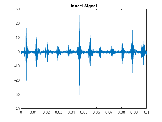
The plot shows periodic impulsive variations in the acceleration measurements over time.

Find the joint moment of second order for both time and frequency

order = [2,2];
momentJ = tfmoment(x_inner1,sr_inner1,order)
momentJ = 3.6253e+08

The resulting moment has only one element, representing the [2,2] time-frequency pair.

Now include the fourth moment for time and frequency. You can also mix orders within a pair. Include a joint moment with a second order for time and a fourth order for frequency. The order matrix contains two columns — the first for time and the second for frequency. Each row contains the order pair to compute.

order = [2,2;2,4;4,4];
momentJ = tfmoment(x_inner1,t_inner1,order);
momentJ(1)
ans = 3.6253e+08
momentJ(2)
ans = 7.9495e+16
momentJ(3)
ans = 4.0886e+17

You can also take the moment using an existing spectrogram. Load the data for a spectrogram which was computed using the same signal and default options. Input this to tfmoment, using the 3-row order matrix already computed.

load tfmoment_data.mat p_inner1_def f_p_def t_p_def
momentJ = tfmoment(p_inner1_def,f_p_def,t_p_def,order);
momentJ(1)
ans = 3.6261e+08
momentJ(2)
ans = 7.9513e+16
momentJ(3)
ans = 4.0896e+17

The joint moments distill a large amount of time and frequency data into a small set of single data points. They represent important, and concise, features that you can use in multiple ways in your application. Possibilities include comparison with health-regime limits and computing moments of segmented data over a period of time to assess long-term degradation.

Input Arguments

collapse all

Time-series signal for which tfmoment returns the moments, specified as a timetable that contains a single variable with a single column. xt must contain increasing, finite row times. If the timetable has missing or duplicate time points, you can fix it using the tips in Clean Timetable with Missing, Duplicate, or Nonuniform Times. xt can be nonuniformly sampled, with the pspectrum constraint that the median time interval and the mean time interval must obey:

1100<Median time intervalMean time interval<100.

Moment orders to return, specified as an n-by-2 matrix with real positive integers.

  • The first column provides the orders of time.

  • The second column provides the orders of frequency.

Example: momentJ = tfmoment(x,[2,2]) specifies the second-order joint moment (variance) of the time-frequency distribution of x.

Example: momentJ = tfmoment(x,[2,2;4,4]) specifies the second and fourth moment orders for both time and frequency of the time-frequency distribution of x.

You can specify any order and number of orders, but low-order moments carry less computational burden and are better suited to real-time applications. You can also use a different order for time than you use for frequency. The first four moment orders correspond to the statistical moments of a data set:

  1. Mean

  2. Variance

  3. Skewness (degree of asymmetry about the mean)

  4. Kurtosis (length of outlier tails in the distribution — a normal distribution has a kurtosis of 3)

For an example, see Find the Joint Time-Frequency Moments of a Time Series.

Time-series signal from which tfmoment returns the moments, specified as a vector.

For an example of a time-series input, see Find the Joint Time-Frequency Moments of a Time Series.

Sample rate of x, specified as positive scalar in hertz when x is uniformly sampled.

Sample-time values, specified as one of the following:

  • duration scalar — time interval between consecutive samples of X.

  • Vector, duration array, or datetime array — time instant or duration corresponding to each element of x.

ts can be nonuniform, with the pspectrum constraint that the median time interval and the mean time interval must obey:

1100<Median time intervalMean time interval<100.

Power spectrogram or spectrum of a signal, specified as a matrix (spectrogram) or a column vector (spectrum). p contains an estimate of the short-term, time-localized power spectrum of a time-series signal. If you specify p, then tfmoment uses p rather than generate its own power spectrogram. For an example, see Find the Joint Time-Frequency Moments of a Time Series.

Frequencies for power spectrogram or spectrum p when p is supplied explicitly to tfmoment, specified as a vector in hertz. The length of fp must be equal to the number of rows in p.

Time information for power spectrogram or spectrum p when p is supplied explicitly to tfmoment, specified as one of the following:

  • Vector of time points, whose data type can be numeric, duration, or datetime. The length of vector tp must be equal to the number of columns in p.

  • duration scalar that represents the time interval in p. The scalar form of tp can be used only when p is a power spectrogram matrix.

  • For the special case where p is a column vector (power spectrum), tp can be a numeric, duration, or datetime scalar representing the time point of the spectrum.

Name-Value Arguments

Specify optional pairs of arguments as Name1=Value1,...,NameN=ValueN, where Name is the argument name and Value is the corresponding value. Name-value arguments must appear after other arguments, but the order of the pairs does not matter.

Before R2021a, use commas to separate each name and value, and enclose Name in quotes.

Example: 'Centralize',false,'FrequencyLimits',[10 100] computes the joint time-frequency moment for the portion of the signal ranging from 10 Hz to 100 Hz.

Centralize-moment option, specified as the comma-separated pair consisting of 'Centralize' and a logical.

  • If Centralize is true, then tfmoment returns the centralized conditional moment by subtracting the conditional mean (which is the first moment) in the computation.

  • If Centralize is false, then tfmoment returns the noncentralized moment, preserving any data offset.

Example: momentJ = tfmoment(x,[2,2],'Centralize',false).

Frequency limits to use, specified as the comma-separated pair consisting of 'FrequencyLimits' and a two-element vector containing lower and upper bounds f1 and f2 in hertz. This specification allows you to exclude a band of data at either end of the spectral range.

Time limits, specified as the comma-separated pair consisting of 'TimeLimits' and a two-element vector containing lower and upper bounds t1 and t2 in the same units as ts, and of the data types:

  • Numeric or duration when fs or a scalar ts are specified, or when ts is a single, double, or duration vector

  • Numeric, duration, or datetime when ts is specified as a datetime vector

This specification allows you to extract a temporal section of data from a longer data set.

Output Arguments

collapse all

Conditional joint moment returned as a vector, the scalar elements of which each represents the joint moment of one of the specified time-frequency order pairs.

momentJ is always a vector, regardless of whether the input data is timetable xt, time-series vector x, or spectrogram data p.

More About

collapse all

Joint Time-Frequency Moments

The joint time-frequency moments of a nonstationary signal comprise a set of time-varying parameters that characterize the signal spectrum as it evolves in time. They are related to the conditional temporal moments and the joint time-frequency moments. The joint time-frequency moment is an integral function of frequency, given time, and marginal distribution. The conditional temporal moment is an integral function of time, given frequency, and marginal distribution. The calculation of the joint time-frequency moment is a double integral that varies both time and frequency [1], [2].

Each moment is associated with a specific order, with the first four orders being the statistical properties of 1) mean, 2) variance, 3) skewness, and 4) kurtosis.

tfmoment computes the joint time-frequency moments of the time-frequency distribution for a signal x, for the orders specified in order. The function performs these steps:

  1. Compute the spectrogram power spectrum, P(t,f), of the input using the pspectrum function and uses it as a time-frequency distribution. If the syntax used supplies an existing P(t,f), then tfmoment uses that instead.

  2. Estimate the joint time-frequency moment tnωm of the signal using, for the noncentralized case:

    tnωm=tnωmP(t,ω)dtdω,

    where m is the order and P(t) is the marginal distribution.

    For the centralized joint time-frequency moment μt,ωn,m(t), the function uses

    μt,ωn,m(t)=1P(ω)(tt1ω)n(ωω1t)mP(t,ω)dtdω,

    where t1ω and ω1t are the first temporal and spectral time-frequency moments.

References

[1] Loughlin, P. J. "What Are the Time-Frequency Moments of a Signal?" Advanced Signal Processing Algorithms, Architectures, and Implementations XI, SPIE Proceedings. Vol. 4474, November 2001.

[2] Loughlin, P., F. Cakrak, and L. Cohen. "Conditional Moment Analysis of Transients with Application to Helicopter Fault Data." Mechanical Systems and Signal Processing. Vol 14, Issue 4, 2000, pp. 511–522.

Extended Capabilities

C/C++ Code Generation
Generate C and C++ code using MATLAB® Coder™.

Version History

Introduced in R2018a