Main Content

tftmoment

Conditional temporal moment of the time-frequency distribution of a signal

Description

Time-frequency moments provide an efficient way to characterize signals whose frequencies change in time (that is, are nonstationary). Such signals can arise from machinery with degraded or failed hardware. Classical Fourier analysis cannot capture the time-varying frequency behavior. Time-frequency distribution generated by short-time Fourier transform (STFT) or other time-frequency analysis techniques can capture the time-varying behavior, but directly treating these distributions as features carries a high computational burden, and potentially introduces unrelated and undesirable feature characteristics. In contrast, distilling the time-frequency distribution results into low-dimension time-frequency moments provides a method for capturing the essential features of the signal in a much smaller data package. Using these moments significantly reduces the computational burden for feature extraction and comparison — a key benefit for real-time operation [1], [2].

The Predictive Maintenance Toolbox™ implements the three branches of time-frequency moment:

  • Conditional spectral moment — tfsmoment

  • Conditional temporal moment — tftmoment

  • Joint time-frequency moment — tfmoment

example

momentT = tftmoment(xt,order) returns the conditional temporal moment of timetable xt as a matrix. The momentT variables provide the temporal moments for the orders you specify in order. The data in xt can be nonuniformly sampled.

example

momentT = tftmoment(x,fs,order) returns the conditional temporal moment of time-series vector x, sampled at rate fs. The moment is returned as a matrix, in which each column represents a temporal moment corresponding to each element in order. With this syntax, x must be uniformly sampled.

example

momentT = tftmoment(x,ts,order) returns the conditional temporal moment of x sampled at the time instants specified by ts in seconds.

  • If ts is a scalar duration, then tftmoment applies it uniformly to all samples.

  • If ts is a vector, then tftmoment applies each element to the corresponding sample in x. Use this syntax for nonuniform sampling.

example

momentT = tftmoment(p,fp,tp,order) returns the conditional temporal moment of a signal whose power spectrogram is p. fp contains the frequencies corresponding to the temporal estimate contained in p. tp contains the vector of time instants corresponding to the centers of the windowed segments used to compute short-time power spectrum estimates. Use this syntax when:

  • You already have the power spectrogram you want to use.

  • You want to customize the options for pspectrum, rather than accept the default pspectrum options that tftmoment applies. Use pspectrum first with the options you want, and then use the output p as input for tftmoment. This approach also allows you to plot the power spectrogram.

momentT = tftmoment(___,Name,Value) specifies additional properties using name-value pair arguments. Options include moment centralization and time-limit specification.

You can use Name,Value with any of the input-argument combinations in previous syntaxes.

example

[momentT,f] = tftmoment(___) returns the frequency vector f associated with the moment matrix in momentT.

You can use f with any of the input-argument combinations in previous syntaxes.

example

tftmoment(___) with no output arguments plots the conditional temporal moment. The plot x-axis is frequency, and the plot y-axis is the corresponding temporal moment.

You can use this syntax with any of the input-argument combinations in previous syntaxes.

Examples

collapse all

Plot the conditional temporal moments of a time series using a plot-only approach and a return-data approach.

Load and plot the data, which consists of simulated vibration measurements for a system with a fault that causes periodic resonances. x is the vector of measurements, and fs is the sampling frequency.

load tftmoment_example x fs

ts=0:1/fs:(length(x)-1)/fs;
figure
subplot(1,2,1)
plot(ts,x)
xlabel('Time in Seconds')
ylabel('Measurement')
title('Simulated Vibration Measurements')

Use the function pspectrum with the 'spectrogram' option to show the frequency content versus time.

subplot(1,2,2)
pspectrum(x,ts,'spectrogram')

Figure contains 2 axes objects. Axes object 1 with title Simulated Vibration Measurements, xlabel Time in Seconds, ylabel Measurement contains an object of type line. Axes object 2 with title Fres = 16.3487 Hz, Tres = 157 ms, xlabel Time (s), ylabel Frequency (Hz) contains an object of type image.

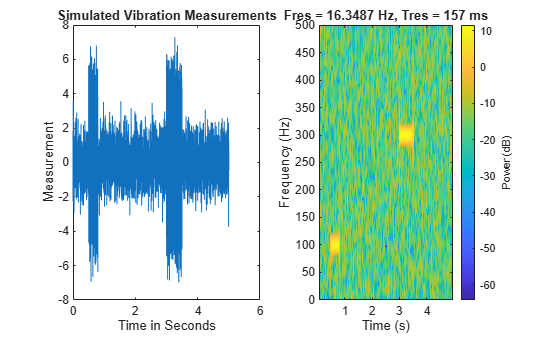
The spectrogram shows that the first burst is at 100 Hz, and the second burst is at 300 Hz. The 300-Hz burst is stronger than the 100-Hz burst by 70 dB.

Plot the second temporal moment (variance), using the plot-only approach with no output arguments and specifying fs.

figure
order = 2;
tftmoment(x,fs,order);title('Second Temporal Moment')

Figure contains an axes object. The axes object with title Second Temporal Moment, xlabel Frequency (Hz), ylabel $ muSubScript t( SuperScript 2 baseline omega )$ contains an object of type line.

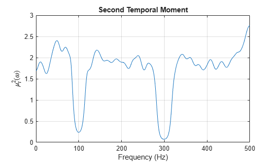
There are two distinct features in the plot at 100 and 300 Hz corresponding to the induced resonances shown by the spectrogram. The moments are much closer in magnitude than the spectral results were.

Now find the first four temporal moments, using the timeline ts that you already constructed. This time, use the form that returns both the moment vectors and the associated frequency vectors. Embed the order array as part of the input argument.

[momentT,f] = tftmoment(x,ts,[1 2 3 4]);

Each column of momentT contains the moment corresponding to one of the input orders.

momentT_1 = momentT(:,1);
momentT_2 = momentT(:,2);
momentT_3 = momentT(:,3);
momentT_4 = momentT(:,4);

Plot the four moments separately to compare the shapes.

figure
subplot(2,2,1)
plot(f,momentT_1)
title('First Temporal Moment — Mean')
xlabel('Frequency in Hz')

subplot(2,2,2)
plot(f,momentT_2)
title('Second Temporal Moment — Variance')
xlabel('Frequency in Hz')

subplot(2,2,3)
plot(f,momentT_3)
title('Third Temporal Moment — Skewness')
xlabel('Frequency in Hz')

subplot(2,2,4)
plot(f,momentT_4)
title('Fourth Temporal Moment — Kurtosis')
xlabel('Frequency in Hz')

Figure contains 4 axes objects. Axes object 1 with title First Temporal Moment — Mean, xlabel Frequency in Hz contains an object of type line. Axes object 2 with title Second Temporal Moment — Variance, xlabel Frequency in Hz contains an object of type line. Axes object 3 with title Third Temporal Moment — Skewness, xlabel Frequency in Hz contains an object of type line. Axes object 4 with title Fourth Temporal Moment — Kurtosis, xlabel Frequency in Hz contains an object of type line.

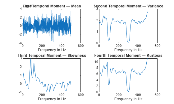
For the data in this example, the second and fourth temporal moments show the clearest features for the faulty resonance.

By default, tfsmoment calls the function pspectrum internally to generate the power spectrogram that tftmoment uses for the moment computation. You can also import an existing power spectrogram for tftmoment to use instead. This capability is useful if you already have a power spectrogram as a starting point, or if you want to customize the pspectrum options by generating the spectrogram explicitly first.

Input a power spectrogram that has already been generated using default options. Compare the resulting temporal-moment plot with one that tftmoment generates using its own pspectrum default options. The results should be the same.

Load the data, which consists of simulated vibration measurements for a system with a fault that causes periodic resonances. p is the previously computed spectrogram, fp and tp are the frequency and time vectors associated with p, x is the original vector of measurements, and fs is the sampling frequency.

load tftmoment_example p fp tp x fs

Determine the second temporal moment using the spectrogram and its associated frequency and time vectors. Plot the moment.

[momentT_p,f_p] = tftmoment(p,fp,tp,2);
figure
subplot(2,1,1)
plot(f_p,momentT_p)
title('Second Temporal Moment using Input Spectrogram ')

Now find and plot the second temporal moments using the original data and sampling rate.

[momentT,f] = tftmoment(x,fs,2);
subplot(2,1,2)
plot(f,momentT)
title('Second Temporal Moment using Measurement Data')

Figure contains 2 axes objects. Axes object 1 with title Second Temporal Moment using Input Spectrogram contains an object of type line. Axes object 2 with title Second Temporal Moment using Measurement Data contains an object of type line.

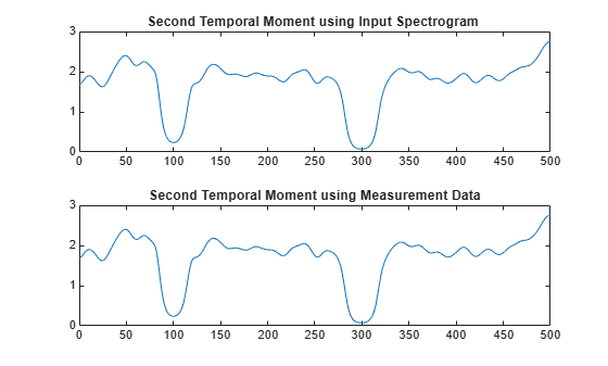
As expected, the plots match since the default pspectrum options were used for both. This result demonstrates the equivalence between the two approaches when there is no customization.

Real-world measurements often come packaged as part of a time-stamped table that records actual time and readings rather than relative times. You can use the timetable format for capturing this data. This example shows how tftmoment operates with a timetable input, in contrast to the data vector inputs used for the other tftmoment examples, such as Plot the Conditional Temporal Moments of a Time Series Vector.

Load the data, which consists of a single timetable (xt_inner1) containing measurement readings and time information for a piece of machinery. Examine the properties of the timetable.

load tfmoment_tdata.mat xt_inner1;
xt_inner1.Properties
ans = 
  TimetableProperties with properties:

             Description: ''
                UserData: []
          DimensionNames: {'Time'  'Variables'}
           VariableNames: {'x_inner1'}
    VariableDescriptions: {}
           VariableUnits: {}
      VariableContinuity: []
                RowTimes: [146484x1 duration]
               StartTime: 0 sec
              SampleRate: 4.8828e+04
                TimeStep: 2.048e-05 sec
                  Events: []
        CustomProperties: No custom properties are set.
      Use addprop and rmprop to modify CustomProperties.

This table consists of dimensions Time and the Variables, where the only variable is x_inner1.

Find the second and fourth conditional temporal moments (order = [2 4]) for the data in the timetable.

order = [2 4];
[momentT_xt_inner1,f] = tftmoment(xt_inner1,order);
size(momentT_xt_inner1)
ans = 1×2

        1024           2

The temporal moments are represented by the columns of momentT_xt_inner1, just as they would be for a moment taken from a time series vector input.

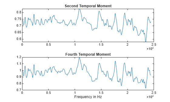
Plot the moments versus returned frequency vector f.

momentT_inner1_2 = momentT_xt_inner1(:,1);
momentT_inner1_4 = momentT_xt_inner1(:,2);

figure
subplot(2,1,1)
plot(f,momentT_inner1_2)
title("Second Temporal Moment")

subplot(2,1,2)
plot(f,momentT_inner1_4)
title("Fourth Temporal Moment")
xlabel('Frequency in Hz')

Figure contains 2 axes objects. Axes object 1 with title Second Temporal Moment contains an object of type line. Axes object 2 with title Fourth Temporal Moment, xlabel Frequency in Hz contains an object of type line.

Input Arguments

collapse all

Time-series signal for which tftmoment returns the moments, specified as a timetable that contains a single variable with a single column. xt must contain increasing, finite row times. If the timetable has missing or duplicate time points, you can fix it using the tips in Clean Timetable with Missing, Duplicate, or Nonuniform Times. xt can be nonuniformly sampled, with the pspectrum constraint that the median time interval and the mean time interval must obey:

1100<Median time intervalMean time interval<100.

For an example of timetable input, see Find the Conditional Temporal Moments of Data Measurements in a Timetable

Moment orders to return, specified as one of the following:

  • Integer — Compute one moment.

  • Vector — Compute multiple moments at once.

Example: momentT = tftmoment(x,2) specifies the second-order temporal moment (variance) of the time-frequency distribution of x.

Example: momentT = tftmoment(x,[1 2 3 4]) specifies the first four moment orders of the time-frequency distribution of x.

You can specify any order and number of orders, but low-order moments carry less computational burden and are better suited to real-time applications. The first four moment orders correspond to the statistical moments of a data set:

  1. Mean ("group delay" for temporal data)

  2. Variance

  3. Skewness (degree of asymmetry about the mean)

  4. Kurtosis (length of outlier tails in the distribution — a normal distribution has a kurtosis of 3)

For examples, see:

Time-series signal from which tftmoment returns the moments, specified as a vector.

For an example of a time-series input, see Plot the Conditional Temporal Moments of a Time Series Vector

Sample rate of x, specified as positive scalar in hertz when x is uniformly sampled.

Sample-time values, specified as one of the following:

  • duration scalar — time interval between consecutive samples of X.

  • Vector, duration array, or datetime array — time instant or duration corresponding to each element of x.

ts can be nonuniform, with the pspectrum constraint that the median time interval and the mean time interval must obey:

1100<Median time intervalMean time interval<100.

Power spectrogram or spectrum of a signal, specified as a matrix (spectrogram) or a column vector (spectrum). p contains an estimate of the short-term, time-localized power spectrum of a time-series signal. If you specify p, then tftmoment uses p rather than generate its own power spectrogram. For an example, see Use a Customized Power Spectrogram to Compute the Conditional Spectral Moment.

Frequencies for power spectrogram or spectrum p when p is supplied explicitly to tftmoment, specified as a vector in hertz. The length of fp must be equal to the number of rows in p.

Time information for power spectrogram or spectrum p when p is supplied explicitly to tftmoment, specified as one of the following:

  • Vector of time points, whose data type can be numeric, duration, or datetime. The length of vector tp must be equal to the number of columns in p.

  • duration scalar that represents the time interval in p. The scalar form of tp can be used only when p is a power spectrogram matrix.

  • For the special case where p is a column vector (power spectrum), tp can be a numeric, duration, or datetime scalar representing the time point of the spectrum.

Name-Value Arguments

Specify optional pairs of arguments as Name1=Value1,...,NameN=ValueN, where Name is the argument name and Value is the corresponding value. Name-value arguments must appear after other arguments, but the order of the pairs does not matter.

Before R2021a, use commas to separate each name and value, and enclose Name in quotes.

Example: 'Centralize',false,'TimeLimits',[20 100] computes the noncentralized conditional temporal moment for the portion of the signal ranging from 20 sec to 100 sec.

Centralize-moment option, specified as the comma-separated pair consisting of 'Centralize' and a logical.

  • If Centralize is true, then tftmoment returns the centralized conditional moment by subtracting the conditional mean (which is the first moment) in the computation.

  • If Centralize is false, then tftmoment returns the noncentralized moment, preserving any data offset.

Example: momentT = tftmoment(x,2,'Centralize',false).

Time limits, specified as the comma-separated pair consisting of 'TimeLimits' and a two-element vector containing lower and upper bounds t1 and t2 in the same units as ts, and of the data types:

  • Numeric or duration when fs or a scalar ts are specified, or when ts is a numeric or duration vector

  • Numeric, duration, or datetime when ts is specified as a datetime vector

This specification allows you to extract a temporal section of data from a longer data set.

Output Arguments

collapse all

Conditional temporal moment returned as a matrix whose columns represent the temporal moments.

momentT is a matrix with one or more columns, regardless of whether the input data is timetable xt, time-series vector x, or spectrogram data p.

Frequencies of moment estimates in hertz, specified as a double vector. For an example, see Plot the Conditional Temporal Moments of a Time Series Vector

More About

collapse all

Conditional Temporal Moments

The conditional temporal moments of a nonstationary signal comprise a set of time-varying parameters that characterize the group delay as it evolves in time. They are related to the conditional spectral moment and the joint time-frequency moments. The conditional spectral moment is an integral function of frequency, given time, and marginal distribution. The conditional temporal moment is an integral function of time, given frequency, and marginal distribution. The joint time-frequency moment is a double integral that varies both time and frequency [1], [2].

Each moment is associated with a specific order, with the first four orders being the statistical properties of 1) mean, 2) variance, 3) skewness, and 4) kurtosis.

tftmoment computes the conditional temporal moments of the time-frequency distribution for a signal x, for the orders specified in order. The function performs these steps:

  1. Compute the spectrogram power spectrum, P(t,f), of the input using the pspectrum function and uses it as a time-frequency distribution. If the syntax used supplies an existing P(t,f), then tftmoment uses that instead.

  2. Estimate the conditional temporal moment tnω of the signal using, for the non-centralized case:

    tnω=1P(ω)tnP(t,ω)dt,

    where m is the order and P(t) is the marginal distribution.

    For the centralized conditional temporal moment μtn(ω), the function uses

    μtn(ω)=1P(ω)(tt1ω)nP(t,ω)dt.

References

[1] Loughlin, P. J. "What are the time-frequency moments of a signal?" Advanced Signal Processing Algorithms, Architectures, and Implementations XI, SPIE Proceedings. Vol. 4474, November 2001.

[2] Loughlin, P., F. Cakrak, and L. Cohen. "Conditional moment analysis of transients with application to helicopter fault data." Mechanical Systems and Signal Processing. Vol 14, Issue 4, 2000, pp. 511–522.

Extended Capabilities

C/C++ Code Generation
Generate C and C++ code using MATLAB® Coder™.

Version History

Introduced in R2018a